- Sign in / Register
- Administration
- Edit profile

The PhET website does not support your browser. We recommend using the latest version of Chrome, Firefox, Safari, or Edge.

Agar Cell Diffusion
All biological cells require the transport of materials across the plasma membrane into and out of the cell. By infusing cubes of agar with a pH indicator, and then soaking the treated cubes in vinegar, you can model how diffusion occurs in cells. Then, by observing cubes of different sizes, you can discover why larger cells might need extra help to transport materials.
- Agar-agar powder
- Digital scale
- Graduated cylinder
- Whisk or fork
- Microwaveable bowl or container at least 500ml in volume
- Microwave (not shown)
- Hot pad or oven mitt
- Heat-safe surface
- pH indicator, such as bromothymol blue or phenolphthalein
- Small glass baking pan or cube-shaped silicone ice-cube molds
- Clear plastic metric ruler
- Sharp knife
- Clear container for immersing agar cubes
- Pencil and notepaper
- White paper or plate

- Measure out 1.6 g of agar-agar and 200 ml water. Mix them together with a whisk or fork in a large microwave-safe bowl.
- Heat the solution in the microwave on high for 30 seconds. Remove to a heat-safe surface using a hot pad or oven mitts, stir, and return to the microwave for 30 seconds. Repeat this process until the mixture boils. (Keep your eye on it as it can boil over very easily!) When done, remove the container, and set it on a trivet or other heat-safe surface.

- Carefully pour the agar solution into silicone ice-cube molds or a small glass baking pan. Make sure the agar block(s) will be at least 3 cm deep when they solidify. If you don’t have enough solution, make more using the ratio of 0.8 g agar-agar powder to 100 ml water.

Place a few millileters of the pH indicator into a small container ( either bromothymol blue or phenolphthalein ). Using a dropper, add a few drops of vinegar. What do you notice?
As an acid, vinegar has a large number of hydrogen ions. When the hydrogen ions come into contact with the pH indicator, the solution changes color.
Fill a clear container with vinegar to a 3-cm depth. Place one agar cube of each size in the vinegar, making sure the blocks are submerged. The untreated blocks (one of each size) will be used for comparison. What do you think will happen to each cube?

Determine the surface area and volume of each cube. To find the surface area, multiply the length of a side of the cube by the width of a side of the cube. This will give you the area of one face of the cube. Multiply this number by 6 (the number of faces on a cube) to determine the total surface area. To find the volume, multiply the length of the cube by its width by its height. Then determine the surface-area-to-volume ratios by dividing the surface area by the volume for each cube.
How will you know if hydrogen ions are moving into the cube? How long do you think it will take the hydrogen ions to diffuse fully into each of the cubes? Why? How would you be able to tell when the vinegar has fully penetrated the cube?
After 5 minutes, remove the cubes from the vinegar with a plastic spoon, and place them on white paper or on a white plate. Compare the treated cubes to the untreated cubes and observe any color changes.
How much vinegar has been absorbed by each treated cube? One way to measure this is to calculate the percentage of the volume of the cube that has been penetrated by the vinegar. (Hint: It may be easier to first consider the volume that has not been penetrated by the vinegar—the portion that has not yet changed color.) Do you want to adjust any of your predictions for the diffusion times? What are your new predictions?

Carefully return all of the treated cubes to the vinegar. Continue checking the vinegar-soaked cubes every 5 minutes by removing them to determine the percentage of the cube that has been penetrated by the vinegar. Continue this process until the vinegar has fully penetrated the cubes. Make a note of the time when this occurs.
What do you notice about the percentage of penetration for each of the cubes at the different time intervals? What relationships do you notice between surface area, volume, surface-area-to-volume ratio, and percentage penetration? What does this say about diffusion as an object gets larger?
Biological cells can only survive if materials can move in and out of them. In this Snack, you used cubes of agar to visualize how diffusion changes depending on the size of the object taking up the material.
Diffusion occurs when molecules in an area of higher concentration move to an area of lower concentration. As hydrogen ions from the vinegar move into the agar cube, the color of the cube changes allowing you to see how far they have diffused. While random molecular motion will cause individual molecules and ions to continue moving back and forth between the cube and the vinegar solution, the overall concentrations will remain in equilibrium, with equal concentrations inside and outside the agar cube.
How did you find the percentage of the cube that was penetrated by the hydrogen ions at the various time intervals? One way to do this is to start with the volume of the cube that has not been penetrated—in other words, the part in the center that has not yet changed color. To determine the volume of this inner cube, measure the length of this inner cube and multiply it by the width and height. Subtract this from the original volume of the cube and you obtain the volume of the cube that has been penetrated. By dividing this number by the original volume and multiplying by 100%, you can determine the percentage penetration for each cube.

You may have noticed that the bigger the vinegar-soaked cube gets, the time it takes for additional vinegar to diffuse into the cube also increases—but not in a linear fashion. In other words, if the cube dimensions are doubled, the time it takes for the hydrogen ions to completely diffuse in more than doubles. When you triple the size, the time to diffuse MUCH more than triples. Why would this happen?
As the size of an object increases, the volume also increases, but by more than you might think. For example, when the cube doubles from a length of 1 cm to a length of 2 cm, the surface area increase by a factor of four, going from 6 cm 2 (1 cm x 1 cm x 6 sides) to 24 cm 2 (2 cm x 2 cm x 6 sides). The volume, though, increases by a factor of eight, increasing from 1 cm 3 (1cm x 1 cm x 1 cm) to 8 cm 3 (2 cm x 2 cm x 2 cm).

Because the volume is increasing at a greater factor than the surface area, the surface-area-to-volume ratio decreases. As the cube size increases, the surface-area-to-volume ratio decreases (click to enlarge the table below). The vinegar can only enter the cube through its surface, so as that ratio decreases, the time it takes for diffusion to occur throughout the whole volume increases significantly.
$$\begin{array}{|c|c|c|c|} \hline \begin{array}{c} \text { Cube Side } \\ \text { Length } \end{array} & \text { Surface Area } & \text { Volume } & \begin{array}{c} \text { Surface-area- } \\ \text { to-volume ratio } \end{array} \\ \hline 1 \mathrm{~cm} & 6 \mathrm{~cm}^2 & 1 \mathrm{~cm}^3 & 6 \mathrm{~cm}^{-1} \\ \hline 2 \mathrm{~cm} & 24 \mathrm{~cm}^2 & 8 \mathrm{~cm}^3 & 3 \mathrm{~cm}^{-1} \\ \hline 3 \mathrm{~cm} & 54 \mathrm{~cm}^2 & 27 \mathrm{~cm}^3 & 2 \mathrm{~cm}^{-1} \\ \hline \end{array}$$
Anything that comes into a cell (such as oxygen and food) or goes out of it (such as waste) must travel across the cell membrane. As cells grow larger, the ratio of surface area to volume decreases dramatically, just like in your agar cubes. Larger cells must still transport materials across their membranes, but have a larger volume to supply and a proportionately smaller surface area through which to do so.
Bacterial cells are fairly small and have a comparatively larger surface-area-to-volume ratio. Eukaryotic cells, such as those in plants and animals, are much larger, but have additional structures to help them conduct the required amount of transport across membranes. A series of membrane-bound structures continuous with the plasma membrane, such as the endoplasmic reticulum, provide additional surface area inside the cell, allowing sufficient transport to occur. Even with these strategies, though, there are upper limits to cell size.
While this Snack investigates how the size of an agar cube impacts diffusion, the shape of each cube remains consistent. Biological cells, however, come in different shapes. To see how different shapes of “cells” affect diffusion rates, try various shapes of agar solids. Ice-cube molds can be found in spherical and rod shapes in addition to cubes. How does the shape impact the surface-area-to-volume ratios?
This Snack fits well into a series of investigations on osmosis and diffusion. The Naked Egg Snack will allow students to explore how concentration gradients power movement of materials into and out of cells. The Cellular Soap Opera Snack will help students consider the types of materials that move through cell membranes.
To help students better understand the concepts of surface area, volume, and surface-area-to-volume ratio, have them build models with plastic centimeter cubes. Physical models can help make these ideas more concrete. Students can also graph class data to better understand the mathematical relationships involved.
If there’s not enough time within a class period for the largest cubes to be fully penetrated by the hydrogen ions present in the vinegar, students can make note of the percentage of the cube that has been penetrated by the vinegar and use that data to extrapolate a result. Alternatively, students in the following period may be able to note the time for the previous class.
Agar-agar comes as a powder and can be purchased online or at markets featuring Asian foods. Unflavored gelatin can be used as a substitute, but is more difficult to handle. To make cubes from gelatin, add boiling water (25% less than the amount recommended on the package) to the gelatin powder, stir, and refrigerate overnight. You may need to experiment with the ratio of water to gelatin to achieve the perfect consistency.
Cabbage juice can be used as an inexpensive alternative to commercial pH indicator solutions. To make cabbage juice indicator, pour boiling water over chopped red cabbage and let it sit for 10 minutes. Strain out the cabbage, and use the remaining purple water to mix with the agar powder.
Related Snacks

STEM Little Explorers
Knowing through exploring.
Home » Articles » STEM » STEM Science » How to Demonstrate Diffusion with Hot and Cold Water

How to Demonstrate Diffusion with Hot and Cold Water
We all need some space sometimes, right that’s true down to a molecular level. molecules don’t like to stay too close together and will try to move to less crowded areas. that process is called diffusion and we will explore all about it in this simple but revealing experiment., article contents.
What is Diffusion?
Have you ever smelled your neighbor’s lunch on your way home? Or smelled someone’s perfume minutes after that person was gone? You experienced the diffusion!
Diffusion is a movement of particles from the area of high concentration to an area of low concentration. It usually occurs in liquids and gases.
Let’s get some complex-sounding terminology out of the way. When talking about diffusion, we often hear something about the concentration gradient (or electrical gradient if looking at electrons). Gradient just means a change in the quantity of a variable over some distance. In the case of concentration gradient, a variable that changes is the concentration of a substance. So we can define the concentration gradient as space over which the concentration of our substance changes.
For example, think of the situation when we spray the air freshener in the room. There is one spot where the concentration of our substance is very high (where we sprayed it initially) and in the rest of the room it is very low (nothing initially). Slowly concentration gradient is diffusing – our freshener is moving through the air. When the concentration gradient is diffused, we reach equilibrium – the state at which a substance is equally distributed throughout a space.

It’s important to note that particles never stop moving , even after the equilibrium is reached. Imagine two parts of the room divided by a line. It may seem like nothing is happening, but particles from both sides are moving back and forth. It’s just that it is an equal probability of them moving from left to right as it’s from right to left. So we can’t notice any net change.
Diffusion is a type of passive transport . That means it doesn’t require energy to start. It happens naturally, without any shaking or stirring.
There is also a facilitated diffusion which happens in the cell membranes when molecules are transported with the help of the proteins.
You may remember hearing about Osmosis and think about how is this different from it. It is actually a very similar concept. Osmosis is just a diffusion through the partially permeable membrane. We talked about it more in our Gummy Bear Osmosis Experiment so definitely check it out.
What causes Diffusion?
Do particles really want to move somewhere less crowded? Well, no, not in the way we would think of it. There is no planning around, just the probability.
All fluids are bound to the same physical laws – studied by Fluid mechanics , part of the physics. We usually think of fluids as liquids, but in fact, air and other types of gas are also fluids ! By definition , fluid is a substance that has no fixed shape and yields easily to external pressure.
Another property of the fluids is that they flow or move around. Molecules in fluids move around randomly and that causes collisions between them and makes them bounce off in different directions.
This random motion of particles in a fluid is called Brownian motion . It was named by the biologist Robert Brown who observed and described the phenomenon in 1827. While doing some experiments with pollen under the microscope, he noticed it wiggles in the water. He concluded that pollen must be alive. Even though his theory was far off, his observation was important in proving the existence of atoms and molecules.
Factors that influence Diffusion
There are several factors that influence the speed of diffusion. The first is the extent of the concentration gradient . The bigger the difference in concentration over the gradient, the faster diffusion occurs.
Another important factor is the distance over which our particles are moving. We can look at it as the size of a container. As you may imagine, with the bigger distance, diffusion is slower, since particles need to move further.
Then we have characteristics of the solvent and substance. The most notable is the mass of the substance and density of the solvent . Heavier molecules move more slowly; therefore, they diffuse more slowly. And it’s a similar case with the density of the solvent. As density increases, the rate of diffusion decreases. It’s harder to move through the denser solvent, therefore our molecules slow down.
And the last factor we will discuss is the temperature . Both heating and cooling change the kinetic energy of the particles in our substance. In the case of heating, we are increasing the kinetic energy of our particles and that makes them move a lot quicker. So the higher the temperature, the higher the diffusion rate.
We will demonstrate the diffusion of food coloring in water and observe how it’s affected by the difference in temperature. Onwards to the experiment!
Materials needed for demonstrating Diffusion

- 2 transparent glasses – Common clear glasses will do the trick. You probably have more than needed around the house. We need one for warm water and one for cold water so we can observe the difference in diffusion.
- Hot and cold water – The bigger the difference in temperature in two glasses, the bigger difference in diffusion will be observed. You can heat the water to near boiling or boiling state and use it as hot water. Use regular water from the pipe as “cold water”. That is enough difference to observe the effects of temperature on diffusion.
- Food coloring – Regular food coloring or some other colors like tempera (poster paint) will do the trick. Color is required to observe the diffusion in our solvent (water). To make it more fun, you can use 2 different colors. Like red for hot and blue for cold.
Instructions for demonstrating diffusion
We have a video on how to demonstrate diffusion at the start of the article so you can check it out if you prefer a video guide more. Or continue reading instructions below if you prefer step by step text guide.
- Take 2 transparent glasses and fill them with the water . In one glass, pour the cold water and in the other hot water. As we mentioned, near-boiling water for hot and regular temperature water from the pipe will be good to demonstrate the diffusion.
- Drop a few drops of food coloring in each cup . 3-4 drops are enough and you should not put too much food color. If you put too much, the concentration of food color will be too large and it will defuse too fast in both glasses.
- Watch closely how the color spreads . You will notice how color diffuses faster in hot water. It will take longer to diffuse if there is more water, less food color and if the water is cooler.
What will you develop and learn
- What is diffusion and how it relates to osmosis
- Factors that influence diffusion
- What is Brownian motion
- How to conduct a science experiment
- That science is fun! 😊
If you liked this activity and are interested in more simple fun experiments, we recommend exploring all about the heat conduction . For more cool visuals made by chemistry, check out Lava lamp and Milk polarity experiment . And if you, like us, find the water fascinating, definitely read our article about many interesting properties of water .
If you’re searching for some great STEM Activities for Kids and Child development tips, you’re in the right place! Check the Categories below to find the right activity for you.

STEM Science
Videos, guides and explanations about STEM Science in a step-by-step way with materials you probably already have at your home. Find new Science ideas.

STEM Technology
Videos, guides and explanations about STEM Technology in a step-by-step way with materials you probably already have at your home. Find new Technology ideas.

STEM Engineering
Videos, guides and explanations about STEM Engineering in a step-by-step way with materials you probably already have at your home. New Engineering ideas!

Videos, guides and explanations about STEM Math in a step-by-step way with materials you probably already have at your home. Find new Mathematics ideas.

Find out all about development psychology topics that you always wanted to know. Here are articles from child psychology and development psychology overall.

First year of Child’s Life
Following a Child’s development every month from its birth. Personal experiences and tips on how to cope with challenges that you will face in parenting.
4 thoughts on “ How to Demonstrate Diffusion with Hot and Cold Water ”
- Pingback: How to Make Colorful Milk Polarity Experiment - STEM Little Explorers
- Pingback: How to make a Lava Lamp | STEM Little Explorers
- Pingback: Learn about pressure with Can Crush Experiment - STEM Little Explorers
- Pingback: Gummy bear Osmosis Experiment - STEM Little Explorers
Leave a Reply Cancel reply
You must be logged in to post a comment.
Get Fresh news from STEM fields
I'm not interested in STEM
Module 4: Diffusion and Osmosis
Diffusion and osmosis.
The cell membrane plays the dual roles of protecting the living cell by acting as a barrier to the outside world, yet at the same time it must allow the passage of food and waste products into and out of the cell for metabolism to proceed. How does the cell carry out these seemingly paradoxical roles? To understand this process you need to understand the makeup of the cell membrane and an important phenomenon known as diffusion.
Diffusion is the movement of a substance from an area of high concentration to an area of low concentration due to random molecular motion. All atoms and molecules possess kinetic energy, which is the energy of movement. It is this kinetic energy that makes each atom or molecule vibrate and move around. (In fact, you can quantify the kinetic energy of the atoms/molecules in a substance by measuring its temperature.) The moving atoms bounce off each other, like bumper cars in a carnival ride. The movement of particles due to this energy is called Brownian motion. As these atoms/molecules bounce off each other, the result is the movement of these particles from an area of high concentration to an area of low concentration. This is diffusion. The rate of diffusion is influenced by both temperature (how fast the particles move) and size (how big they are).

Part 1: Brownian Motion
In this part of the lab, you will use a microscope to observe Brownian motion in carmine red powder, which is a dye obtained from the pulverized guts of female cochineal beetles.
- Glass slide
- Carmine red powder
- Obtain a microscope slide and place a drop of tap water on it.
- Using a toothpick, carefully add a very minuscule quantity of carmine red powder to the drop of water and add a coverslip.
- Observe under scanning, low, and then high power.
Lab Questions
- Describe the activity of the carmine red particles in water.
- If the slide were warmed up, would the rate of motion of the molecules speed up, slow down, or remain the same? Why?
Part 2: Diffusion across a Semipermeable Membrane
Because of its structure, the cell membrane is a semipermeable membrane. This means that SOME substances can easily diffuse through it, like oxygen, or carbon dioxide. Other substances, like glucose or sodium ions, are unable to pass through the cell membrane unless they are specifically transported via proteins embedded in the membrane itself. Whether or not a substance is able to diffuse through a cell membrane depends on the characteristics of the substance and characteristics of the membrane. In this lab, we will make dialysis tubing “cells” and explore the effect of size on a molecule’s ability to diffuse through a “cell membrane.”

The following information might be useful in understanding and interpreting your results in this lab:
- Atomic formula: C 20 H 14 O 4
- Atomic mass: 318.32 g/mol
- Color in acidic solution : Clear
- Color in basic solution: Pink
- Atomic formula: I or I2
- Atomic mass: 126 g/mol
- Atomic formula: (C 6 H 10 O 5 )n
- Atomic mass: HUGE!
- Color in Iodine: Bluish
- Atomic formula: NaOH
- Atomic mass: 40.1 g/mol
- Acid/Base: Base
- 2 pieces of dialysis tubing
- Phenolphthalein
- Starch solution
- Using a wax pencil, label one beaker #1. Label the other beaker #2.
- Fill beaker #1 with 300 ml of tap water, then add 10 drops of 1 M NaOH. Do not spill the NaOH—it is very caustic!
- Fill beaker #2 with 300 ml of tap water, then add iodine drops drop by drop until the solution is bright yellow.
- Now prepare your 2 dialysis tubing “bags.” Seal one end of each dialysis tube by carefully folding the end “hotdog style” 2 times, then “hamburger style” 1 time. Tie the folded portion of the tube securely with string. It is critical that your tubing is tightly sealed, to prevent leaks.
- Add 10 ml of water and three drops of phenolphthalein to one of your dialysis tube bags. Seal the other end of the bag by carefully folding and tying as before.
- Thoroughly rinse the bag containing phenolphthalein, then place it in into the beaker containing the NaOH.
- Add 10 ml of starch solution to the other dialysis tube. Again seal the bag tightly and rinse as above. Place this bag containing the starch solution into beaker #2.
- Let diffusion occur between the bags and the solutions in the beakers.

Record the colors (below) and label contents inside and outside the bags (above):
| Beaker 1 | Beaker 2 | |||
|---|---|---|---|---|
| Initial | Final | Initial | Final | |
| Color inside bag | ||||
| Color outside bag (in beaker) | ||||
- Which substance diffused across the membrane in beaker #1? How do you know?
- Which substance diffused across the membrane in beaker #2? How do you know?
- Why might some ions and molecules pass through the dialysis bag while others might not?
Part 3: Osmosis and the Cell Membrane
Osmosis is the movement of water across a semipermeable membrane (such as the cell membrane). The tonicity of a solution involves comparing the concentration of a cell’s cytoplasm to the concentration of its environment. Ultimately, the tonicity of a solution can be determined by examining the effect a solution has on a cell within the solution.
By definition, a hypertonic solution is one that causes a cell to shrink. Though it certainly is more complex than this, for our purposes in this class, we can assume that a hypertonic solution is more concentrated with solutes than the cytoplasm. This will cause water from the cytoplasm to leave the cell, causing the cell to shrink. If a cell shrinks when placed in a solution, then the solution is hypertonic to the cell.
If a solution is hypotonic to a cell, then the cell will swell when placed in the hypotonic solution. In this case, you can imagine that the solution is less concentrated than the cell’s cytoplasm, causing water from the solution to flow into the cell. The cell swells!
Finally, an isotonic solution is one that causes no change in the cell. You can imagine that the solution and the cell have equal concentrations, so there is no net movement of water molecules into or out of the cell.
In this exercise, you will observe osmosis by exposing a plant cell to salt water.
What do you think will happen to the cell in this environment? Draw a picture of your hypothesis.
- Elodea leaf
- Microscope slide
- 5% NaCl solution
- Remove a leaf from an Elodea plant using the forceps.
- Make a wet mount of the leaf. Use the pond water to make your wet mount.
- Observe the Elodea cells under the compound microscope at high power (400 X) and draw a typical cell below.
- Next, add several drops of 5% salt solution to the edge of the coverslip to allow the salt to diffuse under the coverslip. Observe what happens to the cells (this may require you to search around along the edges of the leaf). Look for cells that have been visibly altered.
Draw a typical cell in both pond and salt water and label the cell membrane and the cell wall.
- What do you see occurring to the cell membrane when the cell was exposed to salt water? Why does this happen?
- Describe the terms hypertonic, hypotonic and isotonic.
- How would your observations change if NaCl could easily pass through the cell membrane and into the cell?
Part 4: Experimental Design
You and your group will design an experiment to determine the relative molecular weights of methylene blue and potassium permanganate. You may use a petri dish of agar, which is a jello-like medium made from a polysaccharide found in the cell walls of red algae. You will also have access to a cork borer and a small plastic ruler.
- 1 petri dish of agar
- Methlylene blue
- Potassium permanganate
Your experiment design should include all of the following portions:
- Experimental design
- Conclusions
- Further questions/other comments
- Biology Labs. Authored by : Wendy Riggs . Provided by : College of the Redwoods. Located at : http://www.redwoods.edu . License : CC BY: Attribution
- Osmotic pressure on blood cells diagram. Authored by : LadyofHats. Located at : https://commons.wikimedia.org/wiki/File:Osmotic_pressure_on_blood_cells_diagram.svg . License : Public Domain: No Known Copyright
The Biology Corner
Biology Teaching Resources

Virtual Diffusion Lab

The diffusion lab has been a yearly activity in my biology class as part of a unit on cells and cell transport. Students fill a bag with starch and water and then submerge it in a solution of iodine and observe what happens. The iodine diffuses across the plastic bag and turns the starch purple.
If students are absent for the lab, they can complete Google Slides that shows the step-by-step process of the investigation. They watch videos showing the set-up and observe a time-lapse video that shows the starch in the bag turn purple. Why does it turn purple?
Iodine in the beaker is a small molecule that can move through the plastic of the bag. When it encounters the starch solution, the color will change to purple. This is an excellent model for how diffusion occurs across semi-permeable membranes.
In the slide activity, a dialysis tube was used instead of a plastic bag because the process does occur faster with the dialysis tube. In class, I use a cheaper version, plastic sandwich bags. Save time and frustration by making the bags ahead of time. Simply put a spoonful of starch in the bag and fill with tap water. Tie the bag like a balloon. Students then place the bag into a beaker with a few drops of iodine .
Google Slides

Other Osmosis Resources
Modeling Osmosis with Deco Cubes
Osmosis Lab
Observing Osmosis in an Egg
Shannan Muskopf
- STEM Ambassadors
- School trusts
- ITE and governors
- Invest in schools
- Student programmes
- Benefits and impact
- Our supporters
- Advertising and sponsorship
- Become a STEM Ambassador
- Request a STEM Ambassador
- Employer information
- Training and support
- STEM Ambassadors Partners
- Working with community groups
- Search icon
- Join the STEM Community
This list provides a range of activities and demonstrations, together with background information and suggested teaching strategies, which explore diffusion. The use of models and analogies here can aid understanding and students should be challenged to use a simple particle model to explain what they observe.
The resources link to the following topics:
- diffusion in terms of the particle model
- diffusion in liquids and gases driven by differences in concentration
- Brownian motion in gases
Visit the secondary science webpage to access all lists: www.nationalstemcentre.org.uk/secondaryscience
Whilst this list provides a source of information and ideas for experimental work, it is important to note that recommendations can date very quickly. Do NOT follow suggestions which conflict with current advice from CLEAPSS, SSERC or recent safety guides. eLibrary users are responsible for ensuring that any activity, including practical work, which they carry out is consistent with current regulations related to health and safety and that they carry an appropriate risk assessment. Further information is provided in our Health and Safety guidance.
Quality Assured Category: Physics Publisher: Longman
Although slightly dated, this pupil book and teacher guide has some really well explained theory and good practicals that fit in with this topic. Each chapter also has a series of good written activities that could be taken and re-purposed in a more up to date way.

Perfumes and Smelling
Quality Assured Category: Science Publisher: Association for Science Education (ASE)
This is a really good set of activities based around perfumes. There are instructions for a perfume circus activity which would make a good starter activity and also for two different ways of making perfume as class practicals. There are full teacher and technician notes and a set of student worksheets.

Diffusion with jelly cubes
In this experiment, students can investigate diffusion by placing agar cubes of varying sizes in acid and observing the colour change. The webpage contains full teacher and technician notes.
Diffusion in liquids
In this experiment, students place colourless crystals of lead nitrate and potassium iodide at opposite sides of a Petri dish of de-ionised water. As these substances dissolve and diffuse towards each other, students can observe clouds of yellow lead iodide forming, demonstrating that diffusion has taken place.
Brownian Motion
Quality Assured Category: Physics Publisher: National STEM Learning Centre and Network
This video shows how to show the movement of particles by Brownian motion. Instead of using the traditional smoke cell, the video shows how Brownian motion can be observed in a suspension containing micrometre diameter polystyrene spheres. Using a microscope and video camera, students can observe the motion of the polystyrene spheres. The video also shows how Brownian motion can be simulated using a vibrating loudspeaker, table tennis balls and a small balloon.

Your browser is not supported
Sorry but it looks as if your browser is out of date. To get the best experience using our site we recommend that you upgrade or switch browsers.
Find a solution
- Skip to main content
- Skip to navigation
- Back to parent navigation item
- Primary teacher
- Secondary/FE teacher
- Early career or student teacher
- Higher education
- Curriculum support
- Literacy in science teaching
- Periodic table
- Interactive periodic table
- Climate change and sustainability
- Resources shop
- Collections
- Remote teaching support
- Starters for ten
- Screen experiments
- Assessment for learning
- Microscale chemistry
- Faces of chemistry
- Classic chemistry experiments
- Nuffield practical collection
- Anecdotes for chemistry teachers
- On this day in chemistry
- Global experiments
- PhET interactive simulations
- Chemistry vignettes
- Context and problem based learning
- Journal of the month
- Chemistry and art
- Art analysis
- Pigments and colours
- Ancient art: today's technology
- Psychology and art theory
- Art and archaeology
- Artists as chemists
- The physics of restoration and conservation
- Ancient Egyptian art
- Ancient Greek art
- Ancient Roman art
- Classic chemistry demonstrations
- In search of solutions
- In search of more solutions
- Creative problem-solving in chemistry
- Solar spark
- Chemistry for non-specialists
- Health and safety in higher education
- Analytical chemistry introductions
- Exhibition chemistry
- Introductory maths for higher education
- Commercial skills for chemists
- Kitchen chemistry
- Journals how to guides
- Chemistry in health
- Chemistry in sport
- Chemistry in your cupboard
- Chocolate chemistry
- Adnoddau addysgu cemeg Cymraeg
- The chemistry of fireworks
- Festive chemistry
- Education in Chemistry
- Teach Chemistry
- On-demand online
- Live online
- Selected PD articles
- PD for primary teachers
- PD for secondary teachers
- What we offer
- Chartered Science Teacher (CSciTeach)
- Teacher mentoring
- UK Chemistry Olympiad
- Who can enter?
- How does it work?
- Resources and past papers
- Top of the Bench
- Schools' Analyst
- Regional support
- Education coordinators
- RSC Yusuf Hamied Inspirational Science Programme
- RSC Education News
- Supporting teacher training
- Interest groups

- More navigation items
Diffusion in liquids
In association with Nuffield Foundation
Demonstrate that diffusion takes place in liquids by allowing lead nitrate and potassium iodide to form lead iodide as they diffuse towards each other in this practical
In this experiment, students place colourless crystals of lead nitrate and potassium iodide at opposite sides of a Petri dish of deionised water. As these substances dissolve and diffuse towards each other, students can observe clouds of yellow lead iodide forming, demonstrating that diffusion has taken place.
This practical activity takes around 30 minutes.
- Eye protection
- White tile or piece of white paper
- Lead nitrate (TOXIC, DANGEROUS FOR THE ENVIRONMENT), 1 crystal
- Potassium iodide, 1 crystal
- Deionised water
Greener alternatives
To reduce the use of toxic chemicals in this experiment you can conduct the experiment in microscale, using drops of water on a laminated sheet, find full instructions and video here, and/or use a less toxic salt than lead nitrate, eg sodium carbonate and barium chloride. More information is available from CLEAPSS.
Health, safety and technical notes
- Read our standard health and safety guidance.
- Wear eye protection throughout.
- Lead nitrate, Pb(NO 3 ) 2 (s), (TOXIC, DANGEROUS FOR THE ENVIRONMENT) – see CLEAPSS Hazcard HC057a .
- Potassium iodide, KI(s) – see CLEAPSS Hazcard HC047b .
- Place a Petri dish on a white tile or piece of white paper. Fill it nearly to the top with deionised water.
- Using forceps, place a crystal of lead nitrate at one side of the petri dish and a crystal of potassium iodide at the other.
- Observe as the crystals begin to dissolve and a new compound is formed between them.

Source: Royal Society of Chemistry
As the crystals of potassium iodide and lead nitrate dissolve and diffuse, they will begin to form yellow lead iodide
Teaching notes
The lead nitrate and potassium iodide each dissolve and begin to diffuse through the water. When the lead ions and iodide ions meet they react to form solid yellow lead iodide which precipitates out of solution.
lead nitrate + potassium iodide → lead iodide + potassium nitrate
Pb(aq) + 2I – (aq) → PbI 2 (s)
The precipitate does not form exactly between the two crystals. This is because the lead ion is heavier and diffuses more slowly through the liquid than the iodide ion.
Another experiment – a teacher demonstration providing an example of a solid–solid reaction – involves the same reaction but in the solid state.
Additional information
This is a resource from the Practical Chemistry project , developed by the Nuffield Foundation and the Royal Society of Chemistry. This collection of over 200 practical activities demonstrates a wide range of chemical concepts and processes. Each activity contains comprehensive information for teachers and technicians, including full technical notes and step-by-step procedures. Practical Chemistry activities accompany Practical Physics and Practical Biology .
The experiment is also part of the Royal Society of Chemistry’s Continuing Professional Development course: Chemistry for non-specialists .
© Nuffield Foundation and the Royal Society of Chemistry
- 11-14 years
- 14-16 years
- Practical experiments
- Physical chemistry
- Reactions and synthesis
Specification
- Precipitation is the reaction of two solutions to form an insoluble salt called a precipitate.
- Motion of particles in solids, liquids and gases.
- Diffusion (Graham's law not required).
Related articles

Help learners master equilibrium and reversible reactions
2024-06-24T06:59:00Z By Emma Owens
Use this poster, fact sheet and storyboard activity to ensure your 14–16 students understand dynamic equilibrium

Non-burning paper: investigate the fire triangle and conditions for combustion
2024-06-10T05:00:00Z By Declan Fleming
Use this reworking of the classic non-burning £5 note demonstration to explore combustion with learners aged 11–16 years

Everything you need to introduce alkenes
2024-06-04T08:22:00Z By Dan Beech
Help your 14–16 learners to master the fundamentals of the reactions of alkenes with these ideas and activities
1 Reader's comment
Only registered users can comment on this article., more experiments.

‘Gold’ coins on a microscale | 14–16 years
By Dorothy Warren and Sandrine Bouchelkia
Practical experiment where learners produce ‘gold’ coins by electroplating a copper coin with zinc, includes follow-up worksheet

Practical potions microscale | 11–14 years
By Kirsty Patterson
Observe chemical changes in this microscale experiment with a spooky twist.

Antibacterial properties of the halogens | 14–18 years
By Kristy Turner
Use this practical to investigate how solutions of the halogens inhibit the growth of bacteria and which is most effective
- Contributors
- Email alerts
Site powered by Webvision Cloud
Sciencing_Icons_Science SCIENCE
Sciencing_icons_biology biology, sciencing_icons_cells cells, sciencing_icons_molecular molecular, sciencing_icons_microorganisms microorganisms, sciencing_icons_genetics genetics, sciencing_icons_human body human body, sciencing_icons_ecology ecology, sciencing_icons_chemistry chemistry, sciencing_icons_atomic & molecular structure atomic & molecular structure, sciencing_icons_bonds bonds, sciencing_icons_reactions reactions, sciencing_icons_stoichiometry stoichiometry, sciencing_icons_solutions solutions, sciencing_icons_acids & bases acids & bases, sciencing_icons_thermodynamics thermodynamics, sciencing_icons_organic chemistry organic chemistry, sciencing_icons_physics physics, sciencing_icons_fundamentals-physics fundamentals, sciencing_icons_electronics electronics, sciencing_icons_waves waves, sciencing_icons_energy energy, sciencing_icons_fluid fluid, sciencing_icons_astronomy astronomy, sciencing_icons_geology geology, sciencing_icons_fundamentals-geology fundamentals, sciencing_icons_minerals & rocks minerals & rocks, sciencing_icons_earth scructure earth structure, sciencing_icons_fossils fossils, sciencing_icons_natural disasters natural disasters, sciencing_icons_nature nature, sciencing_icons_ecosystems ecosystems, sciencing_icons_environment environment, sciencing_icons_insects insects, sciencing_icons_plants & mushrooms plants & mushrooms, sciencing_icons_animals animals, sciencing_icons_math math, sciencing_icons_arithmetic arithmetic, sciencing_icons_addition & subtraction addition & subtraction, sciencing_icons_multiplication & division multiplication & division, sciencing_icons_decimals decimals, sciencing_icons_fractions fractions, sciencing_icons_conversions conversions, sciencing_icons_algebra algebra, sciencing_icons_working with units working with units, sciencing_icons_equations & expressions equations & expressions, sciencing_icons_ratios & proportions ratios & proportions, sciencing_icons_inequalities inequalities, sciencing_icons_exponents & logarithms exponents & logarithms, sciencing_icons_factorization factorization, sciencing_icons_functions functions, sciencing_icons_linear equations linear equations, sciencing_icons_graphs graphs, sciencing_icons_quadratics quadratics, sciencing_icons_polynomials polynomials, sciencing_icons_geometry geometry, sciencing_icons_fundamentals-geometry fundamentals, sciencing_icons_cartesian cartesian, sciencing_icons_circles circles, sciencing_icons_solids solids, sciencing_icons_trigonometry trigonometry, sciencing_icons_probability-statistics probability & statistics, sciencing_icons_mean-median-mode mean/median/mode, sciencing_icons_independent-dependent variables independent/dependent variables, sciencing_icons_deviation deviation, sciencing_icons_correlation correlation, sciencing_icons_sampling sampling, sciencing_icons_distributions distributions, sciencing_icons_probability probability, sciencing_icons_calculus calculus, sciencing_icons_differentiation-integration differentiation/integration, sciencing_icons_application application, sciencing_icons_projects projects, sciencing_icons_news news.
- Share Tweet Email Print
- Home ⋅
- Science Fair Project Ideas for Kids, Middle & High School Students ⋅
Diffusion Lab Experiments

Chemistry Projects for Diffusion in Liquids
Diffusion is a physical phenomenon that occurs everywhere, and we barely notice it or understand how it works. However, a few simple experiments can reveal the mysterious nature of this simple phenomenon.
Preparing for the Experiments
Taking some time to set these experiments up can make your life much easier and allow you to better focus on the results of the experiment. First, grab three glass beakers. Make sure the beakers are transparent. Fill a large pitcher of water or do your experiments near a tap. Also, get three different colors of food dye. To be very precise, you will want a thermometer, but you don't need one unless you are picky. Also have a timer or stopwatch. Finally, make sure you have some way of heating or cooling the water before you start.
Observing Simple Diffusion
This is by far the most simple experiment. However, you'll have to know beforehand that diffusion is the propagation of a substance from an area of high concentration to an area of low concentration, the purpose of which is to reach a state of equilibrium, or a state in which there is an even concentration of a substance across a medium. Now that you know what diffusion is, you need to see it yourself. Take a beaker and fill it with water to around three-quarters. Now, simply pour a small amount of food dye into the water. Observe whether the dye diffuses from a high concentration to a low concentration and try to observe where those two states occur. This will give you a good idea of what diffusion looks like.
Testing How Temperature Affects Diffusion
Now, all your preparation will come to fruition. Fill all three beakers with tap water to around three-quarters filled. The tap water should be around 50 to 60 degrees Fahrenheit, or as close as you can get. Now, cool one beaker by placing it in a refrigerator or similar device. Heat the other beaker with a stove, microwave or, if you have one, a Bunsen burner. You can make the temperatures of all thee beakers whatever you want, really. The important thing is that one is around 20 degrees hotter than another, which is around 20 degrees hotter than another. Finally, put one color of dye in each beaker and observe the diffusion. Your objective in this experiment should be to measure how fast each dye diffuses through each temperature of water. Make sure to write down how fast the dye diffuses in each temperature of water.
Related Articles
Science projects on what liquid freezes faster, science project: the evaporation of fresh water vs...., water density science experiments, fun science experiments with potatoes, how to turn a glass of water with red dye back into..., osmosis egg experiments, heat retention science projects, food coloring experiments, easy 10-minute science projects, osmosis science activities for kids, measuring wet bulb temperature, ideas for fast & easy science fair projects, convection experiments for kids, thermal energy science experiments for kids, how to separate ink from water, how to make salt crystals at home, what is the fastest way to cool a soda for a science..., how to build a hygrometer, how to make a greenhouse for a science project.
About the Author
David Scott has been a firefighter for the Seattle Fire Department's Technical Rescue Team for almost 20 years. He has been writing primarily since 2005, but did author the book, "The White River Ranger District Trail Guide" in 1988. In addition to his work for Demand Studios, Scott spends much of his time writing poetry and a novel.
Find Your Next Great Science Fair Project! GO
Simple Diffusion Experiment

Introduction: Simple Diffusion Experiment

The simple diffusion experiment by Faisal Alwabel in Dhahran Ahliyya Schools MYP 9/C
Step 1: Research Question
How does temperature affect the rate of diffusion?
Step 2: My Hypothesis
•My hypothesis is that:
The lower the temperature of water the slower the diffusion rate inside the water and the longer the time will take, and the higher the temperature the faster diffusion rate inside the water and less time of diffusion in the beaker will take because of the increase of kinetic energy in the particles so they will mix more quickly.
Step 3: Variables (Dependent / Independent / Controlled)
Dependent variable: Rate of diffusion
•Independent variable: Temperature
•Controlled variables: Food coloring drop, time, amount of water for each glass, amount of food coloring
Step 4: Background Research
•What is diffusion? Diffusion is the movement of molecules from a place where they are at a higher concentration to an area with a low concentration, and it works by itself without doing anything to it like shaking and stirring.
•How Does diffusion work? In gases and liquids, the particles move randomly from place to place, and the particles collide with each other or with their container and then the particles are spread to the whole container.
Step 5: Materials

•The materials I will use are:
•* 3 Beakers
•* One cold water, One boiled / hot water, One room temp (30 Celsius)
•* Food coloring
Step 6: Procedure
•1. First of all, I made sure that I had 3 regular spoons for 3 food coloring drops.
•2. Next, I Made sure that every water was in the right temp where one boiled water, one room temp 30 C and one cold water approximately 15 Degrees and they were all 300 ml.
•3. Then I prepared the timer for 5 mins.
•4. After that, I put one food coloring drop for every beaker and start the timer
•5. After 5 minutes, I took photos of all 3 beakers and watched the whole thing.
Step 7: Data

•I saw that the food coloring drip only took 30 seconds to collide with the hot / boiled water, I looked at the room temperature water 30 Degrees C needed approximately 2.5 minutes for the food coloring to collide with it, and finally the 5 minutes finished BUT the food coloring did not collide well with the cold water and had many low concentration areas.
Step 8: Data Analysis
•I found out that there is a huge difference between the three beakers (except for the hot and room temp), I saw that the food coloring and hot water collided really quickly and by that I can say that the rate of diffusion increases as the kinetic energy increases. Similarly, the beaker with the 30 Degrees water was close to the boiled water and all molecules collided with the food coloring but took 2 minutes more. Lastly the cold water, the cold water needed more than 5 minutes to collide but still not all molecules had collided with the food coloring drip and there were many areas with low concentration.
Step 9: Results

•After finishing the experiment, I can start with the results that came out and they are:
•Diffusion rate increases as kinetic energy increases and by that I can say that the boiled / hot water has the highest rate of diffusion because of the kinetic energy inside it.
•The diffusion rate in cold water would be really low because of the small amount of kinetic energy in it so water molecules would not collide with the food coloring.
Step 10: Conclusion
•In conclusion, as you remember my research question was that “How does temperature affect the rate of diffusion?” and I answered it in my data analysis where the rate of diffusion in hot water is high and the rate of diffusion increases as the kinetic energy increases.
•And even my hypothesis was right where I stated that the higher the temperature the faster diffusion rate inside the water and less time of diffusion in the beaker will take because of the increase of the kinetic energy in the particles so they will mix more quickly.
Step 11: Application
•This is a really important subject to study in science because diffusion happens all the time where the diffusion of oxygen and carbon dioxide gas occurs in our lungs, the diffusion of water, salts, and waste that occurs in the kidneys.
Step 12: Evaluation
•The research ATL Skill was really helpful in this experiment wherein background research I had to search for some information to help you understand the process going on and that will happen in the experiment.
Recommendations

Art and Sculpture Contest

Outdoor Life Contest

Woodworking Contest

Sven Elflein About Blog
A practical guide to diffusion models.
The motivation of this blog post is to provide a intuition and a practical guide to train a (simple) diffusion model [Sohl-Dickstein et al. 2015] together with the respective code leveraging PyTorch. If you are interested in a more mathematical description with proofs I can highly recommend [Luo 2022] .
In general, the goal of a diffusion model is to be able to generate novel data after being trained on data points of that distribution.
Here, let’s consider a simple 2D toy dataset provided by scikit-learn to make this example as simple as possible:

Diffusion models define a forward and backward process:
- the forward process gradually adds noise to the data until the original data is indistinguishable (one arrives at a standard normal distribution $N(0, \mathbf{I})$)
- the backward process aims to reverse the forward process, i.e., start from noise and then gradually tries to restore data
To generate new samples by starting from random noise, one aims to learn the backward process.
To be able to start training a model that learns this backward process, we first need to know how to do the forward process.
The forward process adds noise at every step $t$ controlled by parameters \(\{\beta_t\}_{t=1, \dots, T}, \beta_{t-1} < \beta_t, \beta_T = 1\):
As \(t \rightarrow T\) this distribution becomes a multi-variate Gaussian distribution \(\mathcal{N}(0, \mathbf{I})\).
So one starts with the original data samples $x_0$ and then gradually add noise to the samples:

The cool thing about this being Gaussian noise is that instead of simulating this forward process by iteratively sampling noise, one can derive a closed form for the distribution at a certain $t$ given the original data point $x_0$ so one has to only sample noise once:
with $\alpha_t = 1 - \beta_t$ and $\bar{\alpha}_t = \prod_{s = 1}^t \alpha_s$.
Let’s implement this:
Next, we want to train a model that reverses that process.
For this, one can show that the there is also a closed form for the less noisy version $x_{t-1}$ given the next sample $x_t$ and the original sample $x_0$.
and $\epsilon_0 \sim \mathcal{N}(0, \mathbf{I})$ is the noise drawn to perturb the original data $x_0$ 1 .
Obviously, we cannot use this directly to generate new data since this relies on knowing the original datapoint $x_0$ in the first place but we can use it to generate the ground truth data for training a model that does not rely on $\mathbf{x}_0$ and predicts $\epsilon_0$ from the noisy data $\mathbf{x}_t$ and $t$ alone 2 .
Let’s define a small neural network $\epsilon_{\mathbf{\theta}}(\mathbf{x}_t, t)$ where $\mathbf{\theta}$ are the parameters of the network that does just that:
Here, we encode the timestamp of the diffusion process $t$ as a one-hot vector with a single layer and then concatenate this information with the noisy data.
Next up : Training the model to predict the noise. For this, one can just sample $t$’s, use the forward process to generate the noisy sample $x_t$ together with the noise $e_0$, and train the model to reduce the mean squared error between the predicted noise and $e_0$.
After training the model to predict the noise $\epsilon$, we can simply iteratively run the reverse process to predict $\mathbf{x}_{t-1}$ from $x_t$ starting from random noise $\mathbf{x}_T \sim \mathcal{N}(0, \mathbf{I})$ as defined in \eqref{eq:reverse} where we set the mean:
Now, let’s sample new data points and plot them:

We can also inspect the (negative) direction of the predicted noise vector at a particular timestamp $t$ for each position in a grid to visualize the dynamics a sample follows during the reverse process as a vector field:

One can see that as $t \rightarrow 0$ more fine-grained structure emerges that guides the sample to the original data manifold. At $t=T$ samples are guided coarsely towards the center as the signal is still very noisy and hard for the network to predict.
Working on this small dataset already revealed some important things that one has to consider when training diffusion models. In particular, in the beginning when I started to implement this from the paper description, a huge amount of diffusion steps ($T=1000$) were required to yield good results.
Further looking into the literature and appendix of the papers revealed some things that brought down the diffusion steps required to $T=10$:
- It is important to perform linear scaling of the input data into the range $[-1, 1]$. Standardizing the input data (i.e., subtracting the mean and dividing by the standard dev.) as it is usually done for neural networks yielded worse results
- The variance schedule (${\beta_t}_t$) ideally has small changes towards $t=0$ such that the noise is not too much for the network to reconstruct, i.e., it learn fine-grained details of the data. This was already discovered in [Nichol and Dhariwal 2021] , however, it is interesting to see that his insight can be shown from a toy dataset already instead of training expensive image models. Fig. 5 shows how the variance of the forward process $1 - \bar{\alpha}_t$ evolves for when $\beta_t$ is set linear (left), or polynomial (right). The right setting works much better in practice since the perturbation of the input does not happen too fast.

Check out the full notebook which this blog post is based on here .
- Sohl-Dickstein, J., Weiss, E., Maheswaranathan, N., and Ganguli, S. 2015. Deep unsupervised learning using nonequilibrium thermodynamics. International Conference on Machine Learning , PMLR, 2256–2265.
- Luo, C. 2022. Understanding Diffusion Models: A Unified Perspective. .
- Nichol, A.Q. and Dhariwal, P. 2021. Improved Denoising Diffusion Probabilistic Models. International Conference on Machine Learning , PMLR, 8162–8171.
- Ho, J., Jain, A., and Abbeel, P. 2020. Denoising Diffusion Probabilistic Models. Advances in Neural Information Processing Systems 33 , 6840–6851.
This is one possible parameterization of the mean that is most effective based on the experiments in [Ho et al. 2020] . [Luo 2022] summarizes two other paramterizations in the literature, e.g., regressing the mean directly. ↩
Here we treat the variances as fixed. [Nichol and Dhariwal 2021] propose to learn these with an additional objective. ↩
You may also enjoy:
Learning distributions on compact support using normalizing flows --> january 10, 2022 -->, why did my neural network do that --> august 12, 2020 -->.
Practical: Investigating the Rate of Diffusion ( OCR A Level Biology )
Revision note.

Biology & Environmental Systems and Societies
Practical: Investigating the Rate of Diffusion
- It is possible to investigate the effect of certain factors on the rate of diffusion
- Different apparatus can be used to do this, such as Visking tubing and cubes of agar
Practical 1: Investigating the rate of diffusion using visking tubing
- Visking tubing (sometimes referred to as dialysis tubing) is a non-living partially permeable membrane made from cellulose
- Pores in this membrane are small enough to prevent the passage of large molecules (such as starch and sucrose ) but allow smaller molecules (such as glucose ) to pass through by diffusion
- Filling a section of Visking tubing with a mixture of starch and glucose solutions
- Suspending the tubing in a boiling tube of water for a set period of time
- Testing the water outside of the visking tubing at regular intervals for the presence of starch and glucose to monitor whether the diffusion of either substance out of the tubing has occurred
- The results should indicate that glucose, but not starch, diffuses out of the tubing

An example of how to set up an experiment to investigate diffusion
- Comparisons of the glucose concentration between the time intervals can be made using a set of colour standards (produced by known glucose concentrations) or a colorimeter to give a more quantitative set of results
- A graph could be drawn showing how the rate of diffusion changes with the concentration gradient between the inside and outside of the tubing
Practical 2: Investigating the rate of diffusion using agar
- The effect of surface area to volume ratio on the rate of diffusion can be investigated by timing the diffusion of ions through different sized cubes of agar
- Purple agar can be created if it is made up with very dilute sodium hydroxide solution and Universal Indicator
- Alternatively, the agar can be made up with Universal Indicator only
- The acid should have a higher molarity than the sodium hydroxide so that its diffusion can be monitored by a change in colour of the indicator in the agar blocks
- The time taken for the acid to completely change the colour of the indicator in the agar blocks
- The distance travelled into the block by the acid (shown by the change in colour of the indicator) in a given time period (eg. 5 minutes)
- These times can be converted to rates (1 ÷ time taken)
- A graph could be drawn showing how the rate of diffusion (rate of colour change) changes with the surface area to volume ratio of the agar cubes

An example of how to set up an experiment to investigate the effect of changing surface area to volume ratio on the rate of diffusion
When an agar cube (or for example a biological cell or organism) increases in size, the volume increases faster than the surface area, because the volume is cubed whereas the surface area is squared. When an agar cube (or biological cell / organism) has more volume but proportionately less surface area, diffusion takes longer and is less effective. In more precise scientific terms, the greater the surface area to volume ratio , the faster the rate of diffusion !
You've read 0 of your 10 free revision notes
Get unlimited access.
to absolutely everything:
- Downloadable PDFs
- Unlimited Revision Notes
- Topic Questions
- Past Papers
- Model Answers
- Videos (Maths and Science)
Join the 100,000 + Students that ❤️ Save My Exams
the (exam) results speak for themselves:
Did this page help you?
Author: Alistair
Alistair graduated from Oxford University with a degree in Biological Sciences. He has taught GCSE/IGCSE Biology, as well as Biology and Environmental Systems & Societies for the International Baccalaureate Diploma Programme. While teaching in Oxford, Alistair completed his MA Education as Head of Department for Environmental Systems & Societies. Alistair has continued to pursue his interests in ecology and environmental science, recently gaining an MSc in Wildlife Biology & Conservation with Edinburgh Napier University.
Diffusion Course documentation
Unit 1: An Introduction to Diffusion Models
Diffusion course.
and get access to the augmented documentation experience
to get started
Welcome to Unit 1 of the Hugging Face Diffusion Models Course! In this unit, you will learn the basics of how diffusion models work and how to create your own using the 🤗 Diffusers library.
Start this Unit :rocket:
Here are the steps for this unit:
- Make sure you’ve signed up for this course so that you can be notified when new material is released.
- Read through the introductory material below as well as any of the additional resources that sound interesting.
- Check out the Introduction to Diffusers notebook below to put theory into practice with the 🤗 Diffusers library.
- Train and share your own diffusion model using the notebook or the linked training script.
- (Optional) Dive deeper with the Diffusion Models from Scratch notebook if you’re interested in seeing a minimal from-scratch implementation and exploring the different design decisions involved.
- (Optional) Check out this video for an informal run-through the material for this unit.
:loudspeaker: Don’t forget to join the Discord , where you can discuss the material and share what you’ve made in the #diffusion-models-class channel.
What Are Diffusion Models?
Diffusion models are a relatively recent addition to a group of algorithms known as ‘generative models’. The goal of generative modeling is to learn to generate data, such as images or audio, given a number of training examples. A good generative model will create a diverse set of outputs that resemble the training data without being exact copies. How do diffusion models achieve this? Let’s focus on the image generation case for illustrative purposes.

The secret to diffusion models’ success is the iterative nature of the diffusion process. Generation begins with random noise, but this is gradually refined over a number of steps until an output image emerges. At each step, the model estimates how we could go from the current input to a completely denoised version. However, since we only make a small change at every step, any errors in this estimate at the early stages (where predicting the final output is extremely difficult) can be corrected in later updates.
Training the model is relatively straightforward compared to some other types of generative model. We repeatedly 1) Load in some images from the training data 2) Add noise, in different amounts. Remember, we want the model to do a good job estimating how to ‘fix’ (denoise) both extremely noisy images and images that are close to perfect. 3) Feed the noisy versions of the inputs into the model 4) Evaluate how well the model does at denoising these inputs 5) Use this information to update the model weights
To generate new images with a trained model, we begin with a completely random input and repeatedly feed it through the model, updating it each time by a small amount based on the model prediction. As we’ll see, there are a number of sampling methods that try to streamline this process so that we can generate good images with as few steps as possible.
We will show each of these steps in detail in the hands-on notebooks here in unit 1. In unit 2, we will look at how this process can be modified to add additional control over the model outputs through extra conditioning (such as a class label) or with techniques such as guidance. And units 3 and 4 will explore an extremely powerful diffusion model called Stable Diffusion, which can generate images given text descriptions.
Hands-On Notebooks
At this point, you know enough to get started with the accompanying notebooks! The two notebooks here come at the same idea in different ways.
| Chapter | Colab | Kaggle | Gradient | Studio Lab |
|---|---|---|---|---|
| Introduction to Diffusers | ||||
| Diffusion Models from Scratch |
In Introduction to Diffusers , we show the different steps described above using building blocks from the diffusers library. You’ll quickly see how to create, train and sample your own diffusion models on whatever data you choose. By the end of the notebook, you’ll be able to read and modify the example training script to train diffusion models and share them with the world! This notebook also introduces the main exercise associated with this unit, where we will collectively attempt to figure out good ‘training recipes’ for diffusion models at different scales - see the next section for more info.
In Diffusion Models from Scratch , we show those same steps (adding noise to data, creating a model, training and sampling) but implemented from scratch in PyTorch as simply as possible. Then we compare this ‘toy example’ with the diffusers version, noting how the two differ and where improvements have been made. The goal here is to gain familiarity with the different components and the design decisions that go into them so that when you look at a new implementation you can quickly identify the key ideas.
Project Time
Now that you’ve got the basics down, have a go at training one or more diffusion models! Some suggestions are included at the end of the Introduction to Diffusers notebook. Make sure to share your results, training recipes and findings with the community so that we can collectively figure out the best ways to train these models.
Some Additional Resources
The Annotated Diffusion Model is a very in-depth walk-through of the code and theory behind DDPMs with maths and code showing all the different components. It also links to a number of papers for further reading.
Hugging Face documentation on Unconditional Image-Generation for some examples of how to train diffusion models using the official training example script, including code showing how to create your own dataset.
AI Coffee Break video on Diffusion Models: https://www.youtube.com/watch?v=344w5h24-h8
Yannic Kilcher Video on DDPMs: https://www.youtube.com/watch?v=W-O7AZNzbzQ
Found more great resources? Let us know and we’ll add them to this list.
- BiologyDiscussion.com
- Follow Us On:
- Google Plus
- Publish Now
Top 5 Experiments on Diffusion (With Diagram)

ADVERTISEMENTS:
The following points highlight the top five experiments on diffusion. The experiments are: 1. Diffusion of S olid in Liquid 2. Diffusion of Liquid in Liquid 3. Diffusion of Gas in Gas 4. Comparative Rates of Diffusion of Different Solutes 5. Comparative rates of diffusion through different media.
Experiment # 1
Diffusion of s olid in liquid:.
Experiment:
A beaker is almost filled with water. Some crystals of CuSO 4 or KMnO 4 are dropped carefully without disturbing water and is left as such for some time.
Observation:
The water is uniformly coloured, blue in case of CuSO 4 and pink in case of KMnO 4 .
The molecules of the chemicals diffuse gradually from higher concentration to lower concentration and are uniformly distributed after some time. Here, CuSO 4 or KMnO 4 diffuses independently of water and at the same time water diffuses independently of the chemicals.
Experiment # 2
Diffusion of liquid in liquid:.
Two test tubes are taken. To one 30 rim depth of chloroform and to the other 4 mm depth of water are added. Now to the first test tube 4 mm depth of water and to the other 30 mm depth of ether are added (both chloroform and ether form the upper layer).
Ether must be added carefully to avoid disturbance of water. The tubes are stoppered tightly with corks. The position of liquid layers in each test tube is marked and their thickness measured.
The tubes are set aside for some time and the thickness of the liquids in each test tube is recorded at different intervals.
The rate of diffusion of ether is faster than that of chloroform into water as indicated by their respective volumes.
The rate of diffusion is inversely proportional (approximately) to the square root of density of the substance. Substances having higher molecular weights show slower diffusion rates than those having lower molecular weights.
In the present experiment ether (C 2 H 5 -O-G 2 H 5 , J mol. wt. 74) diffuses faster into water than chloroform (CHCI 3 , mol. wt. 119.5). This ratio (74: 119-5) is known as diffusively or coefficient of diffusion.
Experiment # 3
Diffusion of gas in gas:.
One gas jar is filled with CO 2 (either by laboratory method: CaCO 3 + HCL, or by allowing living plant tissue to respire in a closed jar). Another jar is similarly filled with O 2 (either by laboratory method: MnO 2 + KClO 2 , or by allowing green plant tissue to photosynthesize in a dosed jar). The gases may be tested with glowing match stick.
The oxygen jar is then inverted over the mouth of the carbon dioxide jar and made air-tight with grease. It is then allowed to remain for some time. The jars are carefully removed and tested with glowing match stick.
The glowing match sticks flared up in both the jars.
The diffusion of CO 2 and O 2 takes place in both the jars until finally the concentrations are same in both of them making a mixture of CO 2 and O 2 . Hence the glowing match sticks flared up in both the jars.
Experiment # 4
Comparative rates of diffusion of different solutes:.
3.2gm of agar-agar is completely dissolved in 200 ml of boiling water and when partially cooled, 30 drops of methyl red solution and a little of 0.1 N NaOH are added to give an alkaline yellow colour. 3 test tubes are filled three-fourth full with agar mixture and allowed to set.
The agar is covered with 4 ml portion of the following solutions, stoppered tightly and kept in a cool place:
(a) 4 ml of 0-4% methylene blue,
(b) 4 ml of 0.05 N HCl, and (4.2 ml of 0.1ml HCL plus 2 ml of 0-4% methylene blue.
The diffusion of various solutes is recorded in millimeters after 4 hours. The top of the gel should be marked before the above solutions are added.
The rate of diffusion of HCL alone (tube b) is faster compared to the combination of methylene blue and HCl (tube c) and minimum in case of methylene blue alone (tube a).
Different substances like gases, liquids and solutes can diffuse simultaneously and independently at different rates in the same place without interfering each other.
HCL being gaseous in nature and of lower molecular weight can diffuse much faster than methylene blue which is a dye of higher molecular weight having an adsorptive property. Hence in combination, these; two substances diffuse more readily than methylene blue alone.
Experiment # 5
Comparative rates of diffusion through different media:.

- Skip to primary navigation
- Skip to main content
- Skip to primary sidebar

- FREE Experiments
- Kitchen Science
- Climate Change
- Egg Experiments
- Fairy Tale Science
- Edible Science
- Human Health
- Inspirational Women
- Forces and Motion
- Science Fair Projects
- STEM Challenges
- Science Sparks Books
- Contact Science Sparks
- Science Resources for Home and School
Tea bag diffusion!
January 2, 2012 By Emma Vanstone 9 Comments
I love a good cup of tea. In fact, I cannot actually function without one first thing in the morning. If you’re like me, then this investigation is definitely needed in your house so that you can ensure your kids are equipped with the best tea-making skills and have the best scientific knowledge to back up what makes a good cup of tea! This investigation looks at diffusion through the partially permeable membrane of a tea bag.
So firstly, we want to know what type of teabag makes the best drink?
Is it a square, a pyramid or a circle bag?
The activity involves using hot water, so adult supervision is essential.
Teabag diffusion
You’ll need
A stopwatch/timer
A piece of white paper
3 clear glass mugs (you are going to add hot water, so not thin ones that could crack)
Circle, triangle and pyramid tea bags
Thermometer or kettle

1. On the piece of white paper, draw a cross with a marker pen
2. Place one mug over the cross
3. Add the circle teabag
4. Boil water from the kettle and measure out 150ml (if you have a thermometer, you can improve reliability by keeping the temperature constant)
5. Pour over the teabag and start the stopwatch
6. Time how long it takes for the cross to disappear

7. Repeat with the pyramid and square teabag.
8. To make the investigation results more accurate, repeat with each teabag three times.
Record your results in a table

How does the tea diffuse into the water?
So which teabag was quicker?
You should find that the pyramid teabag was the quickest.
Why do you think this is?
As the water is added to the teabag, it causes the tea leaves to move and triggers diffusion of the leaves. Diffusion is defined as the movement of a substance from an area of higher concentration to an area of lower concentration. There are lots of tea molecules in the bag and none outside. The leaves themselves can’t pass through the bag, but their smaller particles containing colour and flavour can (the teabag itself acts as the partially permeable membrane). The addition of heat (from the hot water) to the tea bag causes its molecules to move much faster than at room temperature. This energy is more readily released in a shorter period of time than a tea bag filled with room temperature or cold water. The teabag shape affects the surface area and the pyramid due to its 3D shape providing more surface area for diffusion to take place and more area in the middle for the tea molecules to move around in spreading the colour and flavour.
Ok, so now they know which is the best teabag to use and how to let it brew…so I suggest you ask for a nice cuppa now!
Last Updated on February 23, 2023 by Emma Vanstone
Safety Notice
Science Sparks ( Wild Sparks Enterprises Ltd ) are not liable for the actions of activity of any person who uses the information in this resource or in any of the suggested further resources. Science Sparks assume no liability with regard to injuries or damage to property that may occur as a result of using the information and carrying out the practical activities contained in this resource or in any of the suggested further resources.
These activities are designed to be carried out by children working with a parent, guardian or other appropriate adult. The adult involved is fully responsible for ensuring that the activities are carried out safely.
Reader Interactions
January 06, 2012 at 8:20 pm
What a fun experiment. You always find ways to make the most ordinary things interesting. Thanks for sharing on Monday Madness.
January 06, 2012 at 9:43 pm
January 08, 2012 at 5:37 pm
Interesting especially since all my tea bags are rectangular. I don’t drink it a lot, but and getting to like it more and more. I haven’t tried many brands yet so I will have to start exploring it more. Fun exploration with the kids and I think they probably learned a lot about figuring things out on their own from it.
October 23, 2013 at 2:29 am
awesome job
February 17, 2014 at 8:32 pm
Jah hey thnx.i have learned smthng http://
February 23, 2014 at 12:40 am
Where did the square teabags come from? I have enjoyed tea in that shape but can’t recall what brand. Thanks!
April 29, 2014 at 7:13 pm
thanks! thats really helpful we’re doing a science project on how the shape of the tea bag affects the taste so that was really helpful!!
September 17, 2017 at 11:32 pm
Interesting and helpful. Thanks a lot. Although the cross takes a long time to remove for some reason. Wasnt sure in what marker to use though.
September 29, 2019 at 5:28 pm
WOW i love talking about tea irs so fun wowowowow i learnt science from tea omg wowowowowow omg tea is so interesting
Leave a Reply Cancel reply
Your email address will not be published. Required fields are marked *
Thank you for visiting nature.com. You are using a browser version with limited support for CSS. To obtain the best experience, we recommend you use a more up to date browser (or turn off compatibility mode in Internet Explorer). In the meantime, to ensure continued support, we are displaying the site without styles and JavaScript.
- View all journals
- Explore content
- About the journal
- Publish with us
- Sign up for alerts
- Open access
- Published: 10 August 2024
RS-Dseg: semantic segmentation of high-resolution remote sensing images based on a diffusion model component with unsupervised pretraining
- Zheng Luo 1 ,
- Jianping Pan 1 , 2 , 3 ,
- Yong Hu 4 ,
- Lin Deng 4 ,
- Yimeng Li 1 ,
- Chen Qi 1 &
- Xunxun Wang 1
Scientific Reports volume 14 , Article number: 18609 ( 2024 ) Cite this article
224 Accesses
Metrics details
- Computational science
- Computer science
- Engineering
- Environmental sciences
- Environmental social sciences
Semantic segmentation plays a crucial role in interpreting remote sensing images, especially in high-resolution scenarios where finer object details, complex spatial information and texture structures exist. To address the challenge of better extracting semantic information and ad-dressing class imbalance in multiclass segmentation, we propose utilizing diffusion models for remote sensing image semantic segmentation, along with a lightweight classification module based on a spatial-channel attention mechanism. Our approach incorporates unsupervised pretrained components with a classification module to accelerate model convergence. The diffusion model component, built on the UNet architecture, effectively captures multiscale features with rich contextual and edge information from images. The lightweight classification module, which leverages spatial-channel attention, focuses more efficiently on spatial-channel regions with significant feature information. We evaluated our approach using three publicly available datasets: Postdam, GID, and Five Billion Pixels. In the test of three datasets, our method achieved the best results. On the GID dataset, the overall accuracy was 96.99%, the mean IoU was 92.17%, and the mean F1 score was 95.83%. In the training phase, our model achieved good performance after only 30 training cycles. Compared with other models, our method reduces the number of parameters, improves the training speed, and has obvious performance advantages.
MFCA-Net: a deep learning method for semantic segmentation of remote sensing images

An improved semantic segmentation algorithm for high-resolution remote sensing images based on DeepLabv3+

Joint superpixel and Transformer for high resolution remote sensing image classification
Introduction.
Semantic segmentation of remote sensing images classifies each pixel into different semantic categories. Compared with low-level features, semantic segmentation can directly obtain pixel-level semantic classes and is a crucial intermediate representation for remote sensing image understanding, which can promote intelligent analysis based on remote sensing images. Therefore, it has vital application value in fields such as land use planning, urban construction, and environmental monitoring 1 , 2 , 3 . With the development of remote sensing technology, images with higher spatial resolution can identify smaller and more object categories and details, increasing the seriousness of problems related to the same object with different spectra and different objects with the same spectrum. In multiclass semantic segmentation, an increase in the number of semantic classes will make the training samples of each class sparse, the difference between classes decrease, and the boundaries of ground objects become fuzzy, which brings great challenges to the training and reasoning of the model. How to extract semantic information effectively is the key to semantic segmentation. In an image, the semantic information of an object is usually determined by its local and global context. The model needs to be able to capture this contextual information to better understand the semantic relationships in the image 4 , 5 .
In recent years, the development of deep learning has provided reference experience for extracting information from remote sensing data. Compared with traditional methods, deep learning can better extract spectral-spatial features. Currently, many deep learning models, including classic convolutional neural networks and recently popular vision transformers (ViTs), have been successfully applied to remote sensing image segmentation 6 .
In semantic segmentation tasks, transformers are good at modeling global de-pendencies in images through attention mechanisms and can more accurately classify at the pixel level. However, the computational complexity is high, which is not conducive to processing high-resolution images 7 . CNNs have excellent local feature learning capabilities through convolution and pooling layers and can detect details. Techniques such as separable convolutions and dilated convolutions can also reduce computations. However, they lack representation for long-range pixel correlations and are weaker in extracting global contextual information 8 . Although Atrous Spatial Pyramid Pooling (ASPP) 9 improves this, there is a high computational complexity. Currently, almost all existing deep learning models use CNNs or transformers as a single network structure. The above problems cannot be solved, resulting in a poor segmentation effect. At the same time, to obtain higher accuracy, different modules are stacked and nested for reuse, which complicates the network and lengthens the training cycle. If a CNN and transformer are used together for semantic segmentation, then the segmentation effect will be greatly improved 10 . Therefore, how to combine the advantages of the two for remote sensing image segmentation is a problem worth considering. In recent years, denoising diffusion probabilistic models (DDPMs) have provided a more effective and reliable technical framework for image generation. It has become a vital method in the field of image generation. The diffusion model denoising module takes UNet as the main structure of the model and embeds the transformer self-attention mechanism, position coding and residual module. The self-attention mechanism can capture global information from the entire feature map. Position coding provides the location of the elements in the noise sequence feature to the model. The residual module can prevent the problem of gradient disappearance in the model when the network focuses on local information and can improve the generalization ability of the network. As excellent models for image generation, diffusion models can capture the semantic structure present in the data 11 . Its detail retention capability enables the generation of fine-grained highly detailed images, preserving the context and interrelationships of various objects in the image 12 . In recent years 13 , 14 , 15 , the diffusion model has also been shown to have strong potential in semantic segmentation. Therefore, we hope that this method can be applied to the task of remote sensing image interpretation.
Our goal is to make use of the powerful global information extraction and long-range dependency modeling capabilities of diffusion models to meet the challenges of semantic segmentation of high-resolution remote sensing images. We propose a pretrained feature extractor. The feature extractor is a diffusion model based on the UNet architecture. It is trained in an unsupervised manner on remote sensing images and can extract multiscale features of images. The pre-trained prior knowledge can help the model to achieve better semantic segmentation. These features are then used for semantic segmentation. For the corresponding classification module, we use a spatial-channel attention mechanism that can fuse multiscale features. Notably, it is lightweight, and only the parameters of the classification module are finetuned during segmentation training.
The main contributions of this paper are summarized as follows:
Diffusion models are used for remote sensing image semantic segmentation.
An unsupervised remote sensing image feature extraction model is created using diffusion model.
A lightweight classification module based on a spatial-channel attention mechanism is proposed for processing multiscale features.
Experiments prove that our proposed model and modules have good results.
Our paper is organized as follows: “ Related Work ” section discusses related work in recent years. “ Method ” section details the overall structure of our proposed method. “ Experimental detail ” section adds some details about the experiment. “ Main Experiment ”, “ Ablation experiments ” sections present and discuss the results of comparative experiment and ablation studies. “ Discussion ” section analyzes the conclusion and outlines future research directions. Appendix presents multiscale features.
Related work
Semantic segmentation of high-resolution remote sensing images.
Due to the uniqueness of high-resolution remote sensing images, traditional methods are not ideal for segmentation. In recent years, people have gradually introduced deep learning and made impressive progress. This is mainly due to the automatic feature extraction and end-to-end training of deep learning models. Specifically, the great success of convolutional neural networks in natural image processing has laid the foundation for deep learning in semantic segmentation. It also promoted convolutional network-based semantic segmentation models for remote sensing image analysis. Based on CNNs, researchers proposed the first end-to-end fully convolutional network (FCN) 16 , which replaces the fully connected layer with a convolutional layer to process arbitrarily sized images. Deng 17 fused the spectral index with the FCN model to improve the segmentation effect. Piramanayagam's 18 combination method based on random forest and FCN also achieved high segmentation accuracy. Li 19 used a nonuniform void convolutional network to extract high-level contour features of infrared image targets and fused high-level features of infrared images with detailed features of three scales of RGB images through fusion technology, thus enhancing the feature extraction capability of the network. Guan 20 designed a multiscale feature fusion module in an FCN and used superpixels to optimize the edge, which not only utilized spatial information but also improved the segmentation accuracy. The above model improves the ability of the model to recognize the edge information of the object and effectively integrates the feature information of the high and low layers of the image.Another mainstream framework, the Transformer, consists entirely of an attention mechanism and a feedforward neural network. HRNet 14 is a semantic segmentation network structure proposed by Microsoft Research in 2019 that integrates a transformer structure. The problem of feature resolution downsampling in a U-shaped network is solved, and the segmentation network can retain high-resolution detailed information. SegFormer 13 first used a transformer encoder to build a backbone in the field of semantic segmentation. The hybrid converter module combines convolution and self-attention with both local and global modeling capabilities.
Diffusion models for semantic segmentation
Diffusion models have roots in nonequilibrium thermodynamics 21 , initially concentrating on material diffusion during early research. Over time, their application has extended to diverse domains, including interpolation and prediction in time series data modeling. In the realm of waveform generation, WaveGrad 22 introduced a conditional model that estimates the gradient of data density. This model takes Gaussian white noise as input and iteratively refines input signals using a gradient-based sampler. Within natural language processing, numerous methods grounded in diffusion models have been developed for text generation. DiffuSeq 23 orchestrates diffusion processes in latent space, introducing a novel conditional diffusion model tailored for more intricate text-to-text generation tasks. In the field of computer vision, diffusion models stand as a vibrant area of research, with widespread applications such as image generation 24 , 25 , 26 , 27 , 28 , 29 , 30 , image super-resolution 31 , 32 , 33 , 34 , 35 , image restoration 36 , 37 , 38 , image editing 39 , 40 , and image-to-image translation 41 , 42 , 43 . Palette 44 employed a conditional diffusion model to establish a unified framework for four image generation tasks: colorization, inpainting, decropping, and JPEG restoration. By focusing on synthesizing images with specific desired styles 45 , image translation achieves conditional image generation via DDPM in iterative super-resolution (SR3) 46 . SR3 employs stochastic iterative denoising processes for super-resolution. Imagen Video 47 pioneers cascaded video diffusion models to generate high-definition videos, effectively transferring some methods proven in text-to-image generation tasks to video generation.Researchers have applied diffusion models in segmentation and classification with great potential 48 , 49 , 50 , 51 . Earlier works have focused on representations for zero-shot segmentation 52 or medical images. Wu 53 proposed MedSegDiff-V2, which combines UNet and transformers, outperforming medical image methods. Baranchuk 54 proved that the diffusion model can also be used for semantic segmentation, and the extracted features have rich semantic information. Some studies have explored detection and instance segmentation 26 , 32 .
As shown in Fig. 1 , the whole experiment process is divided into two stages: pre-training and pixel classification. As shown in the left part of Fig. 1 , during the pre-training phase, we input the image into the diffusion model. The diffusion model will degrade and reconstruct the image and learn the semantic information of the images. The most important purpose of pre-training is to enable the model to learn the semantic information of the image, which determines the quality of the features.After the training is completed, the weights of the diffusion model will be frozen, and the diffusion model becomes a feature extractor. We use the diffusion model to extract the image features. According to the set time steps, we will get the multi-scale features under different time steps. After these features are input into the classification module, the pixels are classified with the help of tags, and the result is obtained.We will cover these modules and their procedures in this “ Diffusion Model ” and “ Optimization of the Diffsuion Model ” sections introduce the diffusion and optimization process of the diffusion model. “ Diffusion Model Network Structure ” section shows the network structure of the Diffusion Model, and introduces how the diffusion model carries out feature extraction. “ Feature Extraction ” section introduces the process and details of feature extraction of remote sensing images using diffusion model. “ Lightweight Classification Module ” section The Classification Module dealing with multi-scale features is introduced.

The overall training process of the RS-Dseg.
Diffusion model
Forward diffusion is a forward Markov chain diffusion process that uses a Gaussian noise model. As shown in Fig. 2 , in this process, given the real image \({x}_{0}\) , Gaussian noise with variance \({\beta }_{t}\) is continuously added at a given step, resulting in a noise sequence: \({x}_{1},{x}_{2}\) … After adding enough noise, the image is completely corrupted.

Diagram of the forward and reverse processes.
Its probability distribution is of the form:
The joint distribution of \({x}_{1:T}\) given \({x}_{0}\) is as follows:
If we define \({\alpha }_{t}=1-{\beta }_{t}\) , then \({\prod }_{t=1}^{T}{\alpha }_{i}\) is written for \({\overline{\alpha }}_{t}\) , \({\overline{\alpha }}_{t}\) is the hyperparameter set by the Noise schedule, and (1) can be transformed as follows:
Therefore, Eq. ( 4 ) shows that the value of \({x}_{t}\) depends on the original image \({x}_{0}\) and the random noise \(\epsilon\) . In other words, from the initial value \({x}_{0}\) and the diffusion rate at each step, we can obtain \({x}_{t}\) at any time. When \(t\to \infty\) , \({\beta }_{t}\) continues to increase, and \({\overline{\alpha }}_{t}\) gradually decreases. The mean and variance of \(\epsilon\) are 0 and 1, respectively. Finally, \({x}_{t}\) is an isotropic Gaussian distribution.
The reverse process is the denoising process. we need to learn a model \({p}_{\theta }\) to approximate these conditional probabilities in order to run the reverse diffusion process:
Therefore, the derivation of the following formula is mainly to solve for the mean value. When the variance is given, the Gaussian distribution function of the specified distribution mode can be obtained by solving the mean to simulate the image. Therefore, the derivation of the following formula is used to determine the variance. A standard Gaussian noisy image \({x}_{t}\) is generated from the prior distribution, and then the noise is gradually removed from it by running a learnable backward running Markov chain. The posterior probability of the forward process can be expressed as follows:
According to the Bayes formula and the normal distribution property of Gaussian noise, we can obtain the following:
Therefore, we obtain the a posteriori formula with the parameter \({\alpha }_{t}\) :
Optimization of the diffsuion model
In the forward process, we use randomly generated noise to degrade the image. In the reverse process, we use the corrupted image to estimate the distribution of noise and expect the predicted noise to be close to the real noise. This process can be realized through the iterative training of a neural network. The mathematical principle is to maximize the log-likelihood of the model's predicted distribution, optimizing the cross-entropy between the true distribution \({x}_{0}\) and the predicted distribution \(q\left({x}_{0}\right)\) ,we can obtain the following with Eq. ( 5 ):
We set \({\Sigma }_{\theta }({x}_{t},t)={\sigma }_{t}^{2}I\) , \({\sigma }_{t}^{2}={\widetilde{\beta }}_{t}=\frac{1-{\overline{\alpha }}_{t-1}}{1-{\overline{\alpha }}_{t}}{\beta }_{t}\) , we can obtain the following with Eq. ( 4 ):
where C is a constant that does not depend on θ。From Eq. ( 4 ), we deduce that \({x}_{0}=\frac{{x}_{t}-\sqrt{1-{\overline{a} }_{t}}{\varvec{\epsilon}}}{\sqrt{{\overline{a} }_{t}}}\) . According to the standard Gaussian density function, the mean and variance can be parameterized as follows:
Therefore, at this point, in the backward process, to compute \({\mu }_{t}\) , we need to compute \({x}_{t}\) and \({{\varvec{\epsilon}}}_{t}\) . Therefore, we need to train a neural network to predict the distribution of \({{\varvec{\epsilon}}}_{t}\) . The mean \({\mu }_{t}\) is obtained by predicting the Gaussian noise \({{\varvec{\epsilon}}}_{\theta }\left({x}_{t},t\right)\) from \({x}_{t}\) and \(t\) for each time step. By solving the KL divergence of the multivariate Gaussian distribution, and bring Eq. ( 8 ) into Eq. ( 11 ), we can obtain the following:
Empirically, Ho 25 found that training the diffusion model works better with a simplified objective that ignores the weighting term:
The whole process is to take the input \({x}_{0}\) from \(1\dots T.\) We randomly sample a T in \(t\) . The noise \(\epsilon_{t} \sim {\mathcal{N}}\left( {0,{\varvec{I}}} \right)\) is then sampled from the standard Gaussian distribution. Finally, the objective function \({L}_{t-1}^{\text{simple}}\) is minimized.
As shown in Fig. 2 , the remote sensing images are input into the denoising model as \({x}_{0}\) , and the model is allowed to add noise and reconstruct these remote sensing images. In this way, the distributional noise of the semantic information of these pictures is learned to predict \({\mu }_{t}\) . The whole process does not require labels, and unsupervised pretraining is performed. After completing this process, the denoising model freezes the network parameters. It is subsequently used for feature extraction.
Diffusion model network structure
Figure 3 shows the network structure of the Denoiser. It has a U-shaped structure similar to that of the UNet network. It mainly includes a decoder, an intermediate layer and an encoder. The denoiser mainly consists of a series of Basic I blocks and Basic blocks. At the same time, we connect the encoder to the decoder through the jump connection layer. The denoiser includes the residual structure of the CNN and the self-attention mechanism of the transformer. As shown in Fig. 4 , we used three images with different noise levels as input for model training.

Diffusion model network structure.

Feature extraction and processing.
To help the model better understand and handle the sequence data, we added positional encoding first, as shown in Fig. 3 . This generates a positional code for the noise sequence data, introducing location information into sequence data. Position coding is generated by sine and cosine functions and is related to noise levels. Given the input noise level \(N\_L\) , the dimension of the position encoding is \(dim\) , and \(dim\) is half of the input dimension. First, the position vector \({step}_{i}\) is computed to generate a sequence whose values are in the range [0, 1), representing the proportion of each position relative to the entire sequence. This sequence is mapped to a new range using an exponential function, ensuring large differences in encoding at different locations:
where i represents the position in the sequence and k represents the index in the position vector. \(encodin{g}_{i,j}\) represents the components of each position in the position coding matrix. The sine and cosine values are then concatenated to form the final positional coding vector. At the very beginning of each stage, we add a linear affine layer to embed location information for the feature representation of the network, which helps the model better understand and obtain semantic information for different locations. The Basic I block and Basic block are the main components of the network. The Basic block consists of a GroupNorm (GN) layer, a swish activation function, a dropout layer, and a convolution layer. Basic I replaced the dropout layer with an identity map. We replaced the BatchNorm layer with a GN layer to reduce the impact of BatchSize on the model. The Swish activation function adds nonlinearity to the network, and in deep models, it works better than ReLU 55 . In the first stage of the encoder, to avoid losing considerable semantic information in the initial stage, we do not downsample after the two Basic blocks and Basic I blocks. In other stages, subsampling or attention mechanisms are added at the end. For the input image \(X\in {\mathbb{R}}^{H\times W\times 3}\) , after the first stage, the output is \({F}_{1}^{d}\in {\mathbb{R}}^{H\times W\times 128}\) . From the second stage to the fourth stage, after downsampling at the end, the height and width of the feature are reduced by half, the number of channels is doubled, and the output is \({F}_{n}^{d}\in {\mathbb{R}}^{\left(\frac{H}{{2}^{n}}\right)\times \left(\frac{W}{{2}^{n}}\right)\times \left(128\times n\right)},n=\text{2,3},4\) . In the fifth stage, we do not increase the number of channels of the feature because we consider that when making a jump connection with the feature of the decoder, we increase the number of channels in the second dimension of the feature. The final output of the encoder is \({F}_{5}^{d}\in {\mathbb{R}}^{\left(\frac{H}{16}\right)\times \left(\frac{W}{16}\right)\times 1024}\) .However, the encoder does not increase the number of characteristic channels in stage 5. In the middle layer, the model adjusts \({F}_{5}^{d}\) by a self-attention mechanism.The following is an additional feature representation for the next stage of the decoder:
Then, Q, K, and V can be calculated via convolution:
where \(i\) and \(j\) represent row \(i\) and column \(j\) of \(norm\) , respectively; ( \(m\) , \(n\) ) and K is row \(m\) and column \(n\) of the convolution kernel; and k and l are the height and width of the convolution kernel, respectively. With the Chunk function, Q, K, and V can be obtained. Then, the attention score is calculated:
Finally, the weighted sum of V is calculated using the attention weight:
The output of the middle layer can be expressed as \(F^{m} \in {\mathbb{R}}^{{\left( \frac{H}{16} \right) \times \left( \frac{w}{16} \right) \times 1024}}\) .As shown in Fig. 3 , before the start of each stage of the decoder, the characteristics of each stage of the encoder are combined with the output of the previous stage of the decoder through a jump connection as the input of the next stage of the decoder, \(x_{1} \in {\mathbb{R}}^{{\left( \frac{H}{16} \right) \times \left( \frac{W}{16} \right) \times 2048}}\) .
By connecting the feature graphs of the upsampling and downsampling paths, the low and high-level feature information is combined. This connection helps to retain richer image details and contextual information, avoiding the problem of information loss or disappearing gradients. Information fusion enables the network to focus on both local and global information, improves the model's ability to understand each part of the image, and thus improves the performance of image processing tasks. In addition, the connection feature also helps to introduce more spatial details in the upsampling process, improving the quality of the reconstructed image and the ability to retain details. In the decoder, there are many self-attention mechanisms. This helps the model better understand the semantic information between different features in the noise sequence. The upsampling at the end of each stage causes the size of the feature to become twice the size of the input, gradually returning to the original size of the input.
Feature extraction
After pretraining, the network learns the noise distribution in different diffusion stages. In the reverse stage, the images of different noise levels generated in the forward stage are simulated by the random distribution of Gaussian noise. The whole process does not need backpropagation; it is the result of pretraining. We believe that the generated noise sequence images, due to the powerful global information extraction and remote dependence modeling capabilities of the diffusion model, highlight the importance of different ground objects, thereby helping the model better understand the differences between the various categories. The feature extraction of these images, which contain rich semantic information, helps the network classify pixels better. This is shown in the Appendix.
When performing semantic segmentation, in the reverse process, the feature extractor based on the UNet architecture can perform feature extraction. Figure 4 shows that we feed the trained samples into the denoising model and set the diffusion step in advance. The model gradually diffuses the initial Gaussian noise distribution to approximate the distribution of the sample image. The encoder in the denoising model extracts the image features with the setted diffusion steps. Wele 56 and Dmitry 54 reached a good conclusion on determining diffusion time. Therefore, we directly set the time t to [50, 100, 400]. Figure 4 and the Figure A.1 in Appendix show that images containing different noise levels have different scales of semantic information. The largest difference between the image with diffusion step t = 50 and the other two images is to distinguish the road from the other ground classes in the image. The diffusion step, t = 100, distinguishes natural from unnatural features. T = 400, contains the semantic information of each ground class. The combination of these features can ensure the segmentation accuracy of different land classes. In the Appendix A.1, we show the extracted multiscale features.
Using diffusion models to extract multiscale features is an important process. In the subsequent processing, we directly use these features for classification. Therefore, the extraction and selection of features largely determine the segmentation results. In the ablation experiment, we used different numbers of features for comparison experiments.
Lightweight classification module
For the extracted multiscale features, the proposed classification module needs to classify and upsample them to obtain the results. These features come from images with 3 noise levels and contain different scales and channel numbers, so these features need to be fused and screened. We connect features through convolutional layers and then filter the features through attention mechanisms. Spatial attention and channel attention are weights that adaptively recalibrate features based on context dependencies. Compared with other methods, this method has fewer parameters and lower computational complexity. As shown in Fig. 5 , in addition to the attention mechanism, the whole module contains a small amount of convolution and upsampling, and few parameters are learned. This significantly improves the training speed of the model. and it will be discussed later in the ablation experiment. The experimental results also prove that spatial and channel attention mechanisms are more suitable for feature screening than other methods.

Classification module.
Since the features come from three noise levels, the features of the same size at different noise levels need to first be joined together by convolution. The input features go through a convolutional layer and then enter the channel compression and attention extraction module. In this module, multichannel multiscale features are excited because of their importance. As Fig. 5 shows, this attention module includes spatial squeeze and channel excitation (SSCE) and channel excitation and spatial squeeze (CSSE) 57 .
The SSCE module squeezes the features spatially through fully connected layers and sigmoid activation to obtain excitation weights. The weights are multiplied by the feature scales of each channel's features to capture the importance of different channel features. The extracted multiscale features can be defined as \(F\in {\mathbb{R}}^{H\times W\times C}\) . In SSCE, features are first squeezed spatially through a global pooling layer:
This operation compacts the global spatial information to \({f}_{1}\in {\mathbb{R}}^{1\times 1\times C}\) and then passes through two convolution layers and activation functions:
where \({f}_{2}\in {\mathbb{R}}^{1\times 1\times \left(\frac{C}{2}\right)}\) is the feature after the first convolution and \({f}_{3}\in {\mathbb{R}}^{1\times 1\times C}\) is the feature after two convolutions. Two convolution operations recalibrate the feature on the channel, activating the importance of the different channels after passing through the sigmoid activation function. \({f}_{3}\) acts as a scaling factor to activate the importance of the channel in the original feature:
\({F}_{1}\) represents the features that are given different channel importance after passing through the SSCE module. The CSSE module squeezes the features channelwise using convolutional layers and sigmoid activation to obtain excitation weights. Multiplying the weights with features at different spatial locations allows the capturing of spatial importance. Similarly, for the original feature \(F\in {\mathbb{R}}^{H\times W\times C}\) , passing it through a convolution layer and activation function can be expressed as follows:
\({f}^{1}\in {\mathbb{R}}^{H\times W\times 1}\) , which represents the importance of different spatial locations. \({f}^{1}\) will then act as a scaling factor to rescale the importance of different spatial locations in the original feature:
\({F}_{2}\) represents features that are given different spatial location importance after passing through the CSSE module. Finally, by adding \({F}_{1}\) and \({F}_{2}\) , the treated feature F^* is obtained. As shown in the Fig. 6 , these features that are excited in the channel and spatial positions are used for the final classification convolution and upsampling, and finally, the segmented semantic result is obtained.

Two-branch attention mechanism (SSCE and CSSE).
Experimental detail
Experimental settings.
All experiments were conducted on a 64-bit Windows system equipped with an NVIDIA GeForce RTX 4090 24G GPU. In our experimentation, we first conducted unsupervised pretraining on the training and validation images, excluding the labels, to obtain the feature extractor. During pretraining, we employed the mean squared error (MSE) loss function, with a batch size of 4 and a learning rate of 0.00001. The optimizer utilized was AdamW, with an exponential moving average (EMA) coefficient of 0.9999. In the classification stage, we fixed the batch size at 8 and employed the SGD optimizer with a learning rate of 0.0001.
Evaluation metrics
Accuracy evaluation. We begin from the overall and category perspectives. For the whole, we use the accuracy, average F1 score (Ave.F1), and average IoU (MIoU). These parameters can be represented by the following formula:
Additionally, the F1_score, IoU, recall, and precision are calculated separately for each class. They can be represented by the following formula:
where k is the number of categories.
Postdam : The urban scene classification dataset is provided by ISPRS 66 . The scene is located in the Postdam, which has large buildings, narrow streets and dense settlement structures. The entire dataset contains 6 categories: impervious surfaces, buildings, vegetation, trees, cars, and background. The dataset contains 38 remote sensing images. Among them, 24 images are the training set and 14 images are the test set. We divided the training and validation sets with 20:4 among the 24 remote sensing images. We resize the image to 5120 by 5120 and crop it to 256 by 256. The final dataset has a ratio of 8000:1600:5600. The final quantity ratio is 8000:1600:5600. The RGB values for each category are presented in Table 1 .
GID : The first dataset used in our research is the GID land cover dataset 58 from Wuhan University, which was captured by the Gaofen-2 (GF-2) satellite. We specifically utilized fine classification samples, which consisted of 15 labeled categories. The RGB values for each category are presented in Table 2 and are visualized according to the provided specifications. The dataset comprises 10 processed images with dimensions of 7200 × 6800, which we cropped into 256 × 256 patches.
Main experiment
We compared our model against FCN, ConvNeXt-v2, HRNet, DeepLabv3 + , UNet, SegNeXt, Segformer and FTransUNet. FCN is the first work of deep learning for semantic segmentation and can be adapted to any size of input. Deeplabv3 + and UNet represent early convolutional attention networks. The model can improve the use of features at different levels. The SegFormer model represents another structure transformer, focusing more on the overall message. ConvNeXt-v2 and SegNeXt are novel convolutional attention networks proposed in recent years. Through the information exchange of different branches, HRNet supplements the information loss caused by the reduction in the number of channels. FTransUNet is proposed to provide a robust and effective multimodal fusion backbone for semantic segmentation by integrating both CNN and Vit into one unified fusion framework. The parameters of each model we used in the experiments are shown in Table 3 . Under the premise of ensuring excellent experimental results, our classification head greatly reduces the experimental parameters compared with other models. A decrease in the number of experimental parameters can increase the training speed.
As shown in a and b of Fig. 7 , we recorded the loss values of the seven models on the two datasets over 80 training cycles. Our model (the blue curve) has a lower loss value at the beginning of training than do the other models. It gradually reaches the optimal parameters after approximately 30 training cycles. Other models require approximately 50–60 cycles. The training speed of our model is the fastest among these models.

Loss curve. ( a ): Postdam dataset. ( b ): GID dataset.
Results on the postdam dataset
Table 4 lists the numerical results for each semantic segmentation method. The results show that the proposed RS-Dseg method is superior to other methods in terms of accuracy, MIoU and Ave.F1. UNet with an extended convolutional Deeplabv3 + and decent-encoder structure obtains global context information by extending the receptive field. The experimental results show that a SegFormer with a self-attention mechanism is inferior to our model in long-term dependence modeling. DeepLabv3 + with cavity convolution and residual connections and UNet with a ResNet101 skeleton achieve good results, both reaching 97%. HRNet ranks first among the other models. Compared with HRNet, our method improves the accuracy by 0.68%, the MIoU by 1.83%, and the Ave. F1 by 0.98%. Our approach exceeds the average of the other networks in all three indices by 2.22%, 5.88% and 3.54%. As shown in the third and fourth row of Fig. 8 , Our method is able to extract the edges of features more finely, which is validated in our MIoU values. At the same time, our method also shows a good ability to distinguish similar Categories.

Examples of semantic segmentation results on the Postdam dataset. ( a ): Ours. ( b ): FCN. ( c ): ConvNeXt-v2. ( d ): HRNet. ( e ): Deeplabv3+. ( f ): UNet. ( g ): SegNeXt. ( h ): SegFormer. ( i ): FTransUNet.
Results on GID dataset
Table 5 lists the numerical results for each semantic segmentation method. The results show that the proposed RS-Dseg method is superior to other methods in terms of accuracy, MIoU and Ave.F1. At the same time, with respect to the three indices, the proposed method exceeds the average level of the other models. Our method achieves a 97.00% accuracy, exceeding that of the UNet model by 1.11%. With regard to MIoU, our model achieves a good score of 92.17%, an improvement of 1.48% compared to UNet. With regard to Ave.F1, our model demonstrates an improvement of 0.79% compared to UNet. Neither the transformer-based SegFormer and FTransUNet nor ConvNeXt-v2 and SegNeXt of the new convolutional networks perform as well as our method in this paper.
Compared to other semantic segmentation methods, our proposed model significantly improves object edge identification and integrity. Evaluations show that it increases the average IoU by 5% over others, demonstrating an advantage in accurately extracting edges. Figure 9 illustrates our model and other methods for segmenting the same image. Our model segments class boundaries more precisely, while others exhibit edge blurring. We attribute this to the multiscale features and channel-spatial attention modules. The Attention Mechanism enhances the representation of edge features by scaling the spatial and channel importance of the features. Additionally, our model achieves better object integrity, avoiding fragmentation. For instance, it greatly improves road segmentation accuracy. Compared to other methods, our approach more accurately maintains the coherence and integrity of edges. Future work will further enhance the representation of detailed object edges. For per-class segmentation, we evaluate result using IoU, F1, Precision and Recall. Table 6 shows that, except for artificial grasslands and shrubs, our model outperforms the other models for most of the other classes on most of the metrics. The bolded numbers in-dicate the highest scores among the seven models for that metric and class.

Examples of semantic segmentation results on the GID dataset. ( a ): Ours. ( b ): FCN. ( c ): ConvNeXt-v2. ( d ): HRNet. ( e ): Deeplabv3+. ( f ): UNet. ( g ): SegNeXt. ( h ): SegFormer. ( i ): FTransUNet.
To facilitate a more effective comparison, we choose seven common categories from a total of 15 land classes. Table 7 presents the IoU performance of different methods across these seven categories. Our model consistently outperforms the other models in each category. The average IoU reaches a satisfactorily high score of 93.04%. In comparison, HRNet and UNet, among other models, also achieve average IoU values exceeding 90%. Notably, our model surpasses UNet by approximately 1.7% in average IoU. For example, in the “Transportation” category, other models achieve a minimum IoU of only 64.91%, with the highest reaching 85.22%. Our model surpasses this highest value by 4%. This suggests that in the task of segmenting elongated features, our model demonstrates notably superior performance.
Ablation experiments
In this part, we first discuss the selection of the number of features. The model requires sampling the image through various diffusion steps, and in the decoder of the diffusion model, the size of the features doubles after each upsampling stage. Consequently, a multitude of features can be extracted from a single image. Generally, the more features available, the more beneficial it is for segmenting the model. However, an increase in the number of features results in a higher number of network parameters, thereby escalating the training burden. Hence, the number of features needs careful consideration. Subsequently, we empirically validate each module in this approach, particularly focusing on assessing the effectiveness of DDPM and the space-channel attention mechanism (SCAM).
Different numbers of features
First, we experiment with different numbers of selected features. As mentioned in “Feature Extraction” of “Method”, these features originate from the noise diffusion process. We set diffusion steps so that features of varying scales can be extracted at each step. The number of selected features also determines the classification module parameters. To balance suitable feature numbers and the parameter of classification modules, we tested 4, 5 and 6 feature sets.
According to Table 8 , as the number of features increases, the number of parameters also increases by millions. The average change in accuracy is approximately 0.03%. The MIoU increases by approximately 1% with 6 features, and the Ave.F1 is greater than 96%. The parameter count also increases to approximately fifty-two million. Considering all factors, we selected 4 features for subsequent comparative experiments.As shown in Figure 10 , the segmentation results reveal a few intraclass inconsistencies when using only four features. However, these inconsistencies vanish almost entirely as the number of features increases to six. Despite the differences in categorical consistency, the segmentation boundary and connectivity remain largely unaffected by the number of features. This demonstrates the model's robustness in preserving boundary delineation and connected components with varying feature dimensions. By incrementally enriching the feature space, categorical cohesion improves without compromising the integrity of spatial segmentation. The model thus strikes an effective balance between semantic and structural consistency as feature information increases.

Examples of semantic segmentation results of 4, 5, and 6 features: ( a ) four features; ( b ) five features and ( c ) six features.
Efficiency of moudles
First, we remove two-branch attention mechanism (TBAM)from the classification module and use only DDPM and a small amount of convolution as the model for the first experiment (DDPM). Then, we replace TBAM with ASPP in the classification module, and use DDPM+ASPP as the model of the second experiment to verify whether the features extracted by the feature extractor still need to be further encoded. In addition, to supplement the performance of verifying TBAM, we choose to introduce residual blocks. We selected ResNet-50 as the main model for training, and in another set of experiments, SCAM is added to the end of ResNet-50. We compare the results of the above four sets of experiments with our RS-Dseg.
Table 9 shows the results of each experiment, and our method has the best performance. The performance of the ResNet-50 model has been improved after the addition of SCAM. DDPM results exceeded ResNet and ResNet + SCAM and are slightly lower than DDPM+ SCAM, achieving an Accuracy of 95.14%. Compared with other models in Table 3 , the results of DDPM are also above average, indicating that DDPM is competent for the segmentation task.In addition, following the substitution of SCAM with ASPP, there is a dramatic drop in the performance of model, even performing worse than ResNet-50. DDPM performs worse than DDPM+ SCAM, but better than DDPM+ASPP. This is because the features extracted by the feature extractor can essentially be used for pixel classification without requiring further coding. Additional encoding would degrade segmentation quality. Moreover, from part A.1 of the Appendix, it's evident that these features have been able to represent the categories of ground objects on different scales
Figure 11 shows the result of the segmentation. The combination of (a) gets the best result. Thanks to the feature extractor, these two methods can get accurate results. While (c) is the result of DDPM+ASPP, it can be seen that the quality of segmentation is poor. Using ASPP to re-encode features results in a lot of information being lost, which reduces the accuracy of segmentation. (d) Compared with (e), ResNet-50+ TBAM can better maintain the coherence of long and narrow features due to the presence of space-channel modules.

Examples of semantic segmentation results on the GID dataset ( a ): DDPM + TBAM. ( b ): DDPM. ( c ): DDPM + ASPP. ( d ): ResNet-50. ( e ): ResNet-50 + TBAM.
In this paper, we explore the application of diffusion models in the semantic segmentation of high-resolution remote sensing images, leading to the simplification of existing models for this task. We introduce a lightweight classification module based on spatial-channel attention mechanisms, which enables rapid semantic segmentation by utilizing multiscale features from a pretrained diffusion model. Our experimental results demonstrate that the feature extractor of the unsupervised pretrained diffusion model effectively extracts multiscale features with contextual information. This is due to a prior knowledge of the diffusion model. The lightweight classification module efficiently fuses these features and performs semantic segmentation, significantly reducing the training cycle. These findings highlight the potential of applying diffusion models to remote sensing image semantic segmentation, which can achieve optimal performance compared to current methods. Importantly, in our research, we use labeled images during the segmentation stage but do not utilize them for feature extraction in the diffusion model. In future work, exploring how to leverage the feature extraction capabilities of diffusion models for unsupervised or semi-supervised classification would be valuable.
Data availability
All data generated or analysed during this study are included in this published article [and its supplementary information files].
Karra, K., Kontgis, C., Statman-Weil, Z., Mazzariello, J. C., Mathis, M. & Brumby, S. P. Global land use/land cover with Sentinel 2 and deep learning. In 2021 IEEE International Geoscience and Remote Sensing Symposium IGARSS 4704–4707 (2021) https://doi.org/10.1109/IGARSS47720.2021.9553499
Chen, W., Wu, A. N. & Biljecki, F. Classification of urban morphology with deep learning: Application on urban vitality. Comput. Environ. Urban Syst. 90 , 101706 (2021).
Article Google Scholar
Yuan, Q. et al. Deep learning in environmental remote sensing: Achievements and challenges. Remote Sens. Environ. 241 , 111716 (2020).
Ming, D., Luo, J.-C., Shen, Z., Wang, M. & Sheng, H. Research on high resolution remote sensing image information extraction and target recognition. Sci. Surv. Mapp. 3 , 18–20+3 (2005).
Google Scholar
Yan, Ma. & Kizirbek, G. Research review on image semantic segmentation in high-resolution remote sensing image interpretation. Explor. Comput. Sci. Technol. 17 (07), 1526–1548 (2023).
Vaswani, A. et al . Attention is all you need. In Proceedings of Advances in Neural Information Processing Systems 5998–6008 (2017).
Han, K., Wang, Y., Chen, H., et al . A survey on visual transformer. Preprint arXiv:2012.12556 (2020).
Elngar, A. A. et al. Image classification based on CNN: A survey. J. Cybersecur. Inf. Manag. 6 (1), 18–50 (2021).
Chen, L.-C. et al . Rethinking atrous convolution for semantic image segmentation. Preprint arXiv:1706.05587 (2017).
Yangyi, D., He Kang, Hu. & Qi, H. K. A review of CNN-transformer hybrid model in the field of computer vision. Model. Simul. 12 (4), 3657–3672 (2023).
Valanarasu, J. M. J., Oza, P., Hacihaliloglu, I. et al . Medical transformer: Gated axial-attention for medical image segmentation. In Medical Image Computing and Computer Assisted Intervention–MICCAI 2021: 24th International Conference, Strasbourg, France, September 27–October 1, 2021, Proceedings, Part I 24 . Springer, 36–46 (2021).
Wang, H., Cao, J., Anwer, R. M. et al . Dformer: Diffusion-guided transformer for universal image segmentation. Preprint arXiv:2306.03437 (2023).
Xie, E. et al. SegFormer: Simple and efficient design for semantic segmentation with transformers. Adv. Neural Inf. Process. Syst. 34 , 12077–12090 (2021).
Jingdong, W. et al. Deep high-resolution representation learning for visual recognition. IEEE Trans. Pattern Anal. Mach. Intell. 43 , 3349–3364 (2020).
Roy, A. G., Navab, N., & Wachinger, C. Concurrent spatial and channel ‘squeeze & excitation’in fully convolutional networks. In Medical Image Computing and Computer Assisted Intervention–MICCAI 2018: 21st International Conference, Granada, Spain, September 16-20, 2018, Proceedings, Part I , 421–429 (2018).
Long, J., Shelhamer, E., & Darrell, T. Fully convolutional networks for semantic segmentation. In Proceedings of the IEEE conference on computer vision and pattern recognition 3431–3440 (2015).
Deng, G. H., Gao, F., Luo, Z. P. Research on semantic segmentation of high- resolution remote sensing data based on improved fully convolution neural network. In 4th China High Resolution Earth Observation Conference, Wuhan 1125–1137 (2017).
Piramanayagam, S. et al. Classification of remote sensed images using random forests and deep learning framework. In Image and signal processing for remote sensing XXII Vol. 10004 (SPIE, 2016).
Li, B.-Q. et al. Asymmetric parallel semantic segmentation model based on full convolutional neural network. Acta Electron. Sinica 47 (7), 1058 (2019).
Shen-ke, G. U. A. N. et al. A semantic segmentation algorithm using multi-scale feature fusion with combination of superpixel segmentation. J. Graph. 42 (3), 406 (2021).
Sohl-Dickstein, J., Weiss, E., Maheswaranathan, N., & Ganguli, S. Deep unsupervised learning using non-equilibrium thermodynamics. In Proceedings of ICML 2256–2265 (2015).
Nanxin, C. et al . Wavegrad: Estimating gradients for waveform generation. Preprint arXiv:2009.00713 (2020).
Gong, S. et al . DiffuSeq: Sequence to sequence text generation with diffusion models. In The Eleventh International Conference on Learning Representations . (2022).
Sinha, A., Song, J., Meng, C. & Ermon, S. D2C: Diffusion decoding models for few-shot conditional generation. Adv. Neural Inf. Process. Syst. 34 , 12533–12548 (2021).
Ho, J., Jain, A. & Abbeel, P. Denoising diffusion probabilistic models. Adv. Neural Inf. Process. Syst. 33 , 6840–6851 (2020).
Song, Y. & Ermon, S. Generative modeling by estimating gradients of the data distribution. Adv. Neural Inf. Process. Syst. 32 , 11918–11930 (2019).
Song, Y., Sohl-Dickstein, J., Kingma, D. P., Kumar, A., Ermon, S., & Poole, B. Score-based generative modeling through stochastic differential equations. Advances in neural information processing systems, (2021).
Dhariwal, P. & Nichol, A. Diffusion models beat GANs on image synthesis. Adv. Neural Inf. Process. Syst. 34 , 8780–8794 (2021).
Nichol, A. Q. & Dhariwal, P. Improved denoising diffusion probabilistic models. In Proceedings of ICML , 8162–8171 (2021).
Song, J., Meng, C., & Ermon, S. Denoising diffusion implicit models. In International Conference on Learning Representations (2021).
Daniels, M., Maunu, T. & Hand, P. Score-based generative neural networks for large-scale optimal transport. Adv. Neural Inf. Process. Syst. 34 , 12955–12965 (2021).
Chung, H., Sim, B., & Ye, J. C. Come-closer-diffuse-faster: Accelerating conditional diffusion models for inverse problems through stochastic contraction. In Proceedings of the IEEE/CVF Conference on Computer Vision and Pattern Recognition 12413–12422 (2022).
Kawar, B., Elad, M., Ermon, S. & Song, J. Denoising diffusion restoration models. Adv. Neural Inf. Process. Syst. 35 , 23593–23606 (2022).
Esser, P., Rombach, R., Blattmann, A. & Ommer, B. ImageBART: Bidirectional context with multinomial diffusion for autoregressive image synthesis. Adv. Neural Inf. Process. Syst. 34 , 3518–3532 (2021).
Lugmayr, A., Danelljan, M., Romero, A., Yu, F., Timofte, R., & Van Gool L. RePaint: Inpainting using denoising diffusion probabilistic models. In Proceedings of the IEEE/CVF Conference on Computer Vision and Pattern Recognition , 11461–11471 (2022).
Jing, B., Corso, G., Berlinghieri, R., & Jaakkola, T. Subspace diffusion generative models. Preprint arXiv:2205.01490 (2022).
Avrahami, O., Lischinski, D., & Fried, O. Blended diffusion for text-driven editing of natural images. In Proceedings of the IEEE/CVF Conference on Computer Vision and Pattern Recognition 18208–18218 (2022).
Choi, J., Kim, S., Jeong, Y., Gwon, Y., & Yoon, S. ILVR: Conditioning method for denoising diffusion probabilistic models. In IEEE/CVF International Conference on Computer Vision 14347–14356 (2021).
Meng, C., Song, Y., Song, J., Wu, J., Zhu, J.-Y., & Ermon, S. SDEdit: Guided image synthesis and editing with stochastic differential equations. In International Conference on Learning Representations (2021).
Zhao, M., Bao, F., Li, C. & Zhu, J. EGSDE: Unpaired image-to-image translation via energy-guided stochastic differential equations. Adv. Neural Inf. Process. Syst. 35 , 3609–3623 (2022).
Wang, T., Zhang, T., Zhang, B., Ouyang, H., Chen, D., Chen, Q., & Wen, F. Pretraining is all you need for image-to-image translation. Preprint arXiv:2205.12952 (2022).
Li, B., Xue, K., Liu, B., & Lai, Y.-K. VQBB: image-to-image translation with vector quantized brownian bridge. Preprint arXiv:2205.07680 (2022).
Wolleb, J., Sandkühler, R., Bieder, F., & Cattin, P. C. The Swiss Army knife for image-to-image translation: Multi-task diffusion models. Preprint arXiv:2204.02641 (2022).
Saharia, C., Chan, W., Chang, H., Lee, C., Ho, J., Salimans, T., Fleet, D., & Norouzi, M. Palette: Image-to-image diffusion models. In ACM SIGGRAPH 2022 Conference Proceedings 1–10 (2022).
Sasaki, H., Willcocks, C. G., & Breckon, T. P. UNIT-DDPM: UN-paired image translation with denoising diffusion probabilistic models. Preprint arXiv:2104.05358 (2021).
Chitwan, S. et al. Image super-resolution via iterative refinement. IEEE Trans. Pattern Anal. Mach. Intell. 45 , 4713–4726 (2022).
Ho, J., Chan, W., Saharia, C., Whang, J., Gao, R., Gritsenko, A., Kingma, D. P., Poole, B., Norouzi, M., Fleet, D. J. et al . Imagen video: High definition video generation with diffusion models. Preprint arXiv:2210.02303 (2022).
Brempong, E. A. et al . Denoising pretraining for semantic segmentation. In Proceedings of the IEEE/CVF conference on computer vision and pattern recognition 4175–4186 (2022).
Chen, S., Sun, P., Song, Y., & Luo, P. Diffusiondet: Diffusion model for object detection. In Proceedings of the IEEE/CVF International Conference on Computer Vision 19830–19843 (2023).
Chen, T., et al . A generalist framework for panoptic segmentation of images and videos. In Proceedings of the IEEE/CVF International Conference on Computer Vision 909–919 (2023).
Gu, Z. et al . Diffusioninst: Diffusion model for instance segmentation. Preprint arXiv:2212.02773 (2022).
Burgert, R. et al . Peekaboo: Text to image diffusion models are zero-shot segmentors. Preprint arXiv:2211.13224 (2022).
Wu, J. et al. MedSegDiff: Medical image segmentation with diffusion probabilistic model. In Medical Imaging with Deep Learning (PMLR, 2023).
Baranchuk, D. et al . Label-efficient semantic segmentation with diffusion models. In International Conference on Learning Representations (2021).
Wu, Y., & He, K. Group normalization. In Proceedings of the European conference on computer vision (ECCV) (2018).
Bandara, W. G. C., Nair N. G., Patel, V. M. Remote sensing change detection using denoising diffusion probabilistic models. e-prints arXiv:2206.11892 (2022).
Roy, A. G., Navab, N., Wachinger, C. Concurrent spatial and channel ‘squeeze & excitation’in fully convolutional networks. In Medical Image Computing and Computer Assisted Intervention–MICCAI 2018: 21st International Conference, Granada, Spain, September 16–20, 2018, Proceedings, Part I 421–429 (2018).
Tong, X.-Y. et al. Land-cover classification with high-resolution remote sensing images using transferable deep models. Remote Sens .Environ. 237 , 111–322 (2020).
Long, J., Shelhamer, E., Darrell, T. Fully convolutional networks for semantic segmentation. In Proceedings of the IEEE conference on computer vision and pattern recognition 3431–3440 (2015).
Woo, S., Debnath, S., Hu, R. et al . Convnext v2: Co-designing and scaling convnets with masked autoencoders. In Proceedings of the IEEE/CVF Conference on Computer Vision and Pattern Recognition 16133–16142 (2023).
Wang, J. et al. Deep high-resolution representation learning for visual recognition. IEEE Trans. Pattern Anal. Mach. Intell. 43 , 3349–3364 (2020).
Chen, L-C. et al . Rethinking atrous convolution for semantic image segmentation. Preprint arXiv:1706.05587 (2017).
He, K. et al . Deep residual learning for image recognition. In Proceedings of the IEEE conference on computer vision and pattern recognition 770–778 (2016).
Guo, M. H. et al. Segnext: Rethinking convolutional attention design for semantic segmentation. Adv. Neural Inf. Process. Syst. 35 , 1140–1156 (2022).
Ma, X., Zhang, X., Pun, M.-O. & Liu, M. A multilevel multimodal fusion transformer for remote sensing semantic segmentation. IEEE Trans. Geosci. Remote Sens. 62 , 1–15. https://doi.org/10.1109/TGRS.2024.3373033 (2024).
Rottensteiner, F., Sohn, G., Jung, J., Gerke, M., Baillard, C., Benitez, S., Breitkopf, U. The ISPRS Benchmark on Urban Object Classification and 3D Building Reconstruction. In Proceedings of the ISPRS Annals of the Photogrammetry, Remote Sensing and Spatial Information Sciences, Melbourne, Australia, 25 August–1 September , Vol. I-3, 293–298 (2012).
Download references
Acknowledgements
We thank the reviewers and editors for their insightful comments.
This work was supported in part by the Key R&D Program of Ningxia Autonomous Region: Ecological environment monitoring and platform development of ecological barrier protection system for Helan Mountain (2022CMG02014); the Open Fund of Key Laboratory of Monitoring, Evaluation and Early Warning of Territorial Spatial Planning Implementation, Ministry of Natural Resources (No: LMEE-KF2023001); the Natural Science Foundation of Chong Qing (Nos.CSTB2022NSCQ-MSX1671);in part by the Construction Project of Chongqing Postgraduate Joint Training Base (JDLHPYJD2019004). (Corresponding author: Jianping Pan.)
Author information
Authors and affiliations.
College of Smart City, Chongqing Jiaotong University, Chongqing, 402247, China
Zheng Luo, Jianping Pan, Yimeng Li, Chen Qi & Xunxun Wang
Key Laboratory of Monitoring, Assessment and Early Warning of Land Spatial Planning, Ministry of Natural Resources, Chongqing, 401147, China
Jianping Pan
Technology Innovation Center for Spatio-temporal Information and Equipment of Intelligent City, Ministry of Natural Resources, Chongqing, 401120, China
Chongqing Institute of Surveying and Monitoring for Planning and Natural Resources, Chongqing, 400121, China
Yong Hu & Lin Deng
You can also search for this author in PubMed Google Scholar
Contributions
Conceptualization, Z.L. and J.P.P.; methodology, Z.L.; validation, Z.L.; formal analysis Z.L. Y.M.L. X.X.W. and C.Q. ; resources, Y.H. and L.D. and J.P.P.; writing—original draft preparation, Z.L.; writ-ing—review and editing, Z.L and J.P.P.; All authors have read and agreed to the published version of the manuscript.
Corresponding author
Correspondence to Jianping Pan .
Ethics declarations
Competing interests.
The authors declare no competing interests.
Additional information
Publisher's note.
Springer Nature remains neutral with regard to jurisdictional claims in published maps and institutional affiliations.
Supplementary Information
Supplementary information., rights and permissions.
Open Access This article is licensed under a Creative Commons Attribution-NonCommercial-NoDerivatives 4.0 International License, which permits any non-commercial use, sharing, distribution and reproduction in any medium or format, as long as you give appropriate credit to the original author(s) and the source, provide a link to the Creative Commons licence, and indicate if you modified the licensed material. You do not have permission under this licence to share adapted material derived from this article or parts of it. The images or other third party material in this article are included in the article’s Creative Commons licence, unless indicated otherwise in a credit line to the material. If material is not included in the article’s Creative Commons licence and your intended use is not permitted by statutory regulation or exceeds the permitted use, you will need to obtain permission directly from the copyright holder. To view a copy of this licence, visit http://creativecommons.org/licenses/by-nc-nd/4.0/ .
Reprints and permissions
About this article
Cite this article.
Luo, Z., Pan, J., Hu, Y. et al. RS-Dseg: semantic segmentation of high-resolution remote sensing images based on a diffusion model component with unsupervised pretraining. Sci Rep 14 , 18609 (2024). https://doi.org/10.1038/s41598-024-69022-1
Download citation
Received : 13 May 2024
Accepted : 30 July 2024
Published : 10 August 2024
DOI : https://doi.org/10.1038/s41598-024-69022-1
Share this article
Anyone you share the following link with will be able to read this content:
Sorry, a shareable link is not currently available for this article.
Provided by the Springer Nature SharedIt content-sharing initiative
- Diffusion models
- Pretraining
- Attention mechanism
- Semantic segmentation
By submitting a comment you agree to abide by our Terms and Community Guidelines . If you find something abusive or that does not comply with our terms or guidelines please flag it as inappropriate.
Quick links
- Explore articles by subject
- Guide to authors
- Editorial policies
Sign up for the Nature Briefing: Anthropocene newsletter — what matters in anthropocene research, free to your inbox weekly.

Unveiling Hermes 3: The First Fine-Tuned Llama 3.1 405B Model is on Lambda’s Cloud
Try Hermes 3 for free with the New Lambda Chat Completions API and Lambda Chat.
Introducing hermes 3: a new era for llama fine-tuning.
We are thrilled to announce our partner Nous Research’s launch of Hermes 3 — the first full-parameter fine-tune of Meta's groundbreaking Llama 3.1 405B model , trained on Lambda’s 1-Click Cluster. Designed for the open-source community, Hermes 3 is a neutrally-aligned generalist model with exceptional reasoning capabilities, now available for free through the new Lambda Chat Completions API and Lambda Chat interface. Powered by an 8-node Lambda 1-Click Cluster , Nous Research achieved outstanding results in just a few short weeks. Hermes 3 meets or exceeds Llama 3.1 Instruct on Open Source LLM benchmarks (see table below).
"Lambda’s 1-Click Clusters make the experience of renting and using a multi-node cluster as simple and easy as renting and using a single node,"
-Jeffrey Quesnelle, co-founder of Nous Research
Hermes 3: A uniquely unlocked, uncensored, and steerable model
Hermes 3 is the latest advancement in Nous Research's series of models, which have been downloaded over 33 million times. This instruct-tuned model is specifically designed to be flexible and adept at following instructions. It excels in complex role-playing and creative writing, offering users more immersive character portrayals, deeper simulations, and unexpected fictional experiences.

In addition to its creative capabilities, Hermes 3 is an invaluable tool for professionals requiring advanced reasoning and decision-making abilities. Its strategic planning and operational decision-making features include function-calling, step-labeled reasoning, and more.
Optimized for efficiency
Hermes 3 was meticulously trained using synthesized data and supervised fine-tuning on Meta’s Llama 3.1 405B base model. This was followed by reinforcement learning from human feedback (RLHF) and finally, quantization using Neural Magic’s FP8 method. This optimization effectively reduces the model's VRAM and disk requirements by approximately 50%, allowing it to run on a single node.
“Since the start of my journey in AI I wanted to bring about the realization of an open source frontier level model that aligns to you, the user - not some corporation or higher authority before the user. Today, with Hermes 3 405B, we've achieved that goal, a model that is frontier level, but truly aligned to you. Thanks to our hard work on data synthesis and post training research, we were able to make a dataset that is fully synthetic over almost a year in the making to train Hermes 3 - and will be releasing much more to come.”
-Teknium, cofounder of Nous Research
For those seeking dedicated access and flexibility, Hermes 3 can run on a single node (available on-demand on Lambda’s Cloud ), or quickly scale to a multi-node 1-Click Cluster for further fine-tuning using Lambda's scalable cluster infrastructure.
T ry Hermes 3 for free - for a limited time!
We’re excited to offer the AI/ML community free access to Hermes 3 through Lambda’s new Chat Completions API, fully compatible with the OpenAI API. It provides endpoints for creating completions, chat completions and listing models. No complex setup is required—simply generate a Cloud API key from Lambda’s dashboard ( sign-up ) and start exploring with our documentation ’s help. For a more interactive experience, we’re also providing a simple chat interface: try your prompts in Lambda Chat !
More on the Deep Learning Blog:

Hugging Face x Lambda: Whisper Fine-Tuning Event
Lambda is thrilled to team up with Hugging Face , a community platform that enables users to build,...

Fine tuning Meta's LLaMA 2 on Lambda GPU Cloud
This blog post provides instructions on how to fine tune Llama 2 models on Lambda Cloud using a...

How to fine tune stable diffusion: how we made the text-to-pokemon model at Lambda
Stable Diffusion is great at many things, but not great at everything, and getting results in a...
AI Tools 101
Flux by black forest labs: the next leap in text-to-image models. is it better than midjourney.
Table Of Contents

Black Forest Labs , the team behind the groundbreaking Stable Diffusion model, has released Flux – a suite of state-of-the-art models that promise to redefine the capabilities of AI-generated imagery. But does Flux truly represent a leap forward in the field, and how does it stack up against industry leaders like Midjourney? Let's dive deep into the world of Flux and explore its potential to reshape the future of AI-generated art and media.
The Birth of Black Forest Labs
Before we delve into the technical aspects of Flux, it's crucial to understand the pedigree behind this innovative model. Black Forest Labs is not just another AI startup; it's a powerhouse of talent with a track record of developing foundational generative AI models. The team includes the creators of VQGAN, Latent Diffusion, and the Stable Diffusion family of models that have taken the AI art world by storm.

Black Forest Labs Open-Source FLUX.1
With a successful Series Seed funding round of $31 million led by Andreessen Horowitz and support from notable angel investors, Black Forest Labs has positioned itself at the forefront of generative AI research. Their mission is clear: to develop and advance state-of-the-art generative deep learning models for media such as images and videos, while pushing the boundaries of creativity, efficiency, and diversity.
Introducing the Flux Model Family
Black Forest Labs has introduced the FLUX.1 suite of text-to-image models, designed to set new benchmarks in image detail, prompt adherence, style diversity, and scene complexity. The Flux family consists of three variants, each tailored to different use cases and accessibility levels:
- FLUX.1 [pro] : The flagship model, offering top-tier performance in image generation with superior prompt following, visual quality, image detail, and output diversity. Available through an API, it's positioned as the premium option for professional and enterprise use.
- FLUX.1 [dev] : An open-weight, guidance-distilled model for non-commercial applications. It's designed to achieve similar quality and prompt adherence capabilities as the pro version while being more efficient.
- FLUX.1 [schnell] : The fastest model in the suite, optimized for local development and personal use. It's openly available under an Apache 2.0 license, making it accessible for a wide range of applications and experiments.
I'll provide some unique and creative prompt examples that showcase FLUX.1's capabilities. These prompts will highlight the model's strengths in handling text, complex compositions, and challenging elements like hands.
- Artistic Style Blending with Text: “Create a portrait of Vincent van Gogh in his signature style, but replace his beard with swirling brush strokes that form the words ‘Starry Night' in cursive.”

- Dynamic Action Scene with Text Integration: “A superhero bursting through a comic book page. The action lines and sound effects should form the hero's name ‘FLUX FORCE' in bold, dynamic typography.”

- Surreal Concept with Precise Object Placement: “Close-up of a cute cat with brown and white colors under window sunlight. Sharp focus on eye texture and color. Natural lighting to capture authentic eye shine and depth.”

These prompts are designed to challenge FLUX.1's capabilities in text rendering, complex scene composition, and detailed object creation, while also showcasing its potential for creative and unique image generation.
Technical Innovations Behind Flux
At the heart of Flux's impressive capabilities lies a series of technical innovations that set it apart from its predecessors and contemporaries:
Transformer-powered Flow Models at Scale
All public FLUX.1 models are built on a hybrid architecture that combines multimodal and parallel diffusion transformer blocks, scaled to an impressive 12 billion parameters. This represents a significant leap in model size and complexity compared to many existing text-to-image models.
The Flux models improve upon previous state-of-the-art diffusion models by incorporating flow matching, a general and conceptually simple method for training generative models. Flow matching provides a more flexible framework for generative modeling, with diffusion models being a special case within this broader approach.
To enhance model performance and hardware efficiency, Black Forest Labs has integrated rotary positional embeddings and parallel attention layers. These techniques allow for better handling of spatial relationships in images and more efficient processing of large-scale data.
Architectural Innovations
Let's break down some of the key architectural elements that contribute to Flux's performance:
- Hybrid Architecture : By combining multimodal and parallel diffusion transformer blocks, Flux can effectively process both textual and visual information, leading to better alignment between prompts and generated images.
- Flow Matching : This approach allows for more flexible and efficient training of generative models. It provides a unified framework that encompasses diffusion models and other generative techniques, potentially leading to more robust and versatile image generation.
- Rotary Positional Embeddings : These embeddings help the model better understand and maintain spatial relationships within images, which is crucial for generating coherent and detailed visual content.
- Parallel Attention Layers : This technique allows for more efficient processing of attention mechanisms, which are critical for understanding relationships between different elements in both text prompts and generated images.
- Scaling to 12B Parameters : The sheer size of the model allows it to capture and synthesize more complex patterns and relationships, potentially leading to higher quality and more diverse outputs.
Benchmarking Flux: A New Standard in Image Synthesis

https://blackforestlabs.ai/announcing-black-forest-labs/
Black Forest Labs claims that FLUX.1 sets new standards in image synthesis, surpassing popular models like Midjourney v6.0, DALL·E 3 (HD), and SD3-Ultra in several key aspects:
- Visual Quality : Flux aims to produce images with higher fidelity, more realistic details, and better overall aesthetic appeal.
- Prompt Following : The model is designed to adhere more closely to the given text prompts, generating images that more accurately reflect the user's intentions.
- Size/Aspect Variability : Flux supports a diverse range of aspect ratios and resolutions, from 0.1 to 2.0 megapixels, offering flexibility for various use cases.
- Typography : The model shows improved capabilities in generating and rendering text within images, a common challenge for many text-to-image models.
- Output Diversity : Flux is specifically fine-tuned to preserve the entire output diversity from pretraining, offering a wider range of creative possibilities.
Flux vs. Midjourney: A Comparative Analysis

Now, let's address the burning question: Is Flux better than Midjourney ? To answer this, we need to consider several factors:
Image Quality and Aesthetics
Both Flux and Midjourney are known for producing high-quality, visually stunning images. Midjourney has been praised for its artistic flair and ability to create images with a distinct aesthetic appeal. Flux, with its advanced architecture and larger parameter count, aims to match or exceed this level of quality.
Early examples from Flux show impressive detail, realistic textures, and a strong grasp of lighting and composition. However, the subjective nature of art makes it difficult to definitively claim superiority in this area. Users may find that each model has its strengths in different styles or types of imagery.
Prompt Adherence
One area where Flux potentially edges out Midjourney is in prompt adherence. Black Forest Labs has emphasized their focus on improving the model's ability to accurately interpret and execute on given prompts. This could result in generated images that more closely match the user's intentions, especially for complex or nuanced requests.
Midjourney has sometimes been criticized for taking creative liberties with prompts, which can lead to beautiful but unexpected results. Flux's approach may offer more precise control over the generated output.
Speed and Efficiency
With the introduction of FLUX.1 [schnell], Black Forest Labs is targeting one of Midjourney's key advantages: speed. Midjourney is known for its rapid generation times, which has made it popular for iterative creative processes. If Flux can match or exceed this speed while maintaining quality, it could be a significant selling point.
Accessibility and Ease of Use
Midjourney has gained popularity partly due to its user-friendly interface and integration with Discord. Flux, being newer, may need time to develop similarly accessible interfaces. However, the open-source nature of FLUX.1 [schnell] and [dev] models could lead to a wide range of community-developed tools and integrations, potentially surpassing Midjourney in terms of flexibility and customization options.
Technical Capabilities
Flux's advanced architecture and larger model size suggest that it may have more raw capability in terms of understanding complex prompts and generating intricate details. The flow matching approach and hybrid architecture could allow Flux to handle a wider range of tasks and generate more diverse outputs.
Ethical Considerations and Bias Mitigation
Both Flux and Midjourney face the challenge of addressing ethical concerns in AI-generated imagery, such as bias, misinformation, and copyright issues. Black Forest Labs' emphasis on transparency and their commitment to making models widely accessible could potentially lead to more robust community oversight and faster improvements in these areas.
Code Implementation and Deployment
Using flux with diffusers.
Flux models can be easily integrated into existing workflows using the Hugging Face Diffusers library . Here's a step-by-step guide to using FLUX.1 [dev] or FLUX.1 [schnell] with Diffusers:
- First, install or upgrade the Diffusers library:
- Then, you can use the FluxPipeline to run the model:
This code snippet demonstrates how to load the FLUX.1 [dev] model, generate an image from a text prompt, and save the result.
Deploying Flux as an API with LitServe
For those looking to deploy Flux as a scalable API service, Black Forest Labs provides an example using LitServe, a high-performance inference engine. Here's a breakdown of the deployment process:
Define the model server:
This code sets up a LitServe API for Flux, including model loading, request handling, image generation, and response encoding.
Start the server:
Use the model api:.
You can test the API using a simple client script:
Key Features of the Deployment
- Serverless Architecture : The LitServe setup allows for scalable, serverless deployment that can scale to zero when not in use.
- Private API : You can deploy Flux as a private API on your own infrastructure.
- Multi-GPU Support : The setup is designed to work efficiently across multiple GPUs.
- Quantization : The code demonstrates how to quantize the model to 8-bit precision, allowing it to run on less powerful hardware like NVIDIA L4 GPUs.
- CPU Offloading : The enable_model_cpu_offload() method is used to conserve GPU memory by offloading parts of the model to CPU when not in use.
Practical Applications of Flux
The versatility and power of Flux open up a wide range of potential applications across various industries:
- Creative Industries : Graphic designers, illustrators, and artists can use Flux to quickly generate concept art, mood boards, and visual inspirations.
- Marketing and Advertising : Marketers can create custom visuals for campaigns, social media content, and product mockups with unprecedented speed and quality.
- Game Development : Game designers can use Flux to rapidly prototype environments, characters, and assets, streamlining the pre-production process.
- Architecture and Interior Design : Architects and designers can generate realistic visualizations of spaces and structures based on textual descriptions.
- Education : Educators can create custom visual aids and illustrations to enhance learning materials and make complex concepts more accessible.
- Film and Animation : Storyboard artists and animators can use Flux to quickly visualize scenes and characters, accelerating the pre-visualization process.
The Future of Flux and Text-to-Image Generation
Black Forest Labs has made it clear that Flux is just the beginning of their ambitions in the generative AI space. They've announced plans to develop competitive generative text-to-video systems, promising precise creation and editing capabilities at high definition and unprecedented speed.
This roadmap suggests that Flux is not just a standalone product but part of a broader ecosystem of generative AI tools. As the technology evolves, we can expect to see:
- Improved Integration : Seamless workflows between text-to-image and text-to-video generation, allowing for more complex and dynamic content creation.
- Enhanced Customization : More fine-grained control over generated content, possibly through advanced prompt engineering techniques or intuitive user interfaces.
- Real-time Generation : As models like FLUX.1 [schnell] continue to improve, we may see real-time image generation capabilities that could revolutionize live content creation and interactive media.
- Cross-modal Generation : The ability to generate and manipulate content across multiple modalities (text, image, video, audio) in a cohesive and integrated manner.
- Ethical AI Development : Continued focus on developing AI models that are not only powerful but also responsible and ethically sound.
Conclusion: Is Flux Better Than Midjourney?
The question of whether Flux is “better” than Midjourney is not easily answered with a simple yes or no. Both models represent the cutting edge of text-to-image generation technology, each with its own strengths and unique characteristics.
Flux, with its advanced architecture and emphasis on prompt adherence, may offer more precise control and potentially higher quality in certain scenarios. Its open-source variants also provide opportunities for customization and integration that could be highly valuable for developers and researchers.
Midjourney , on the other hand, has a proven track record, a large and active user base, and a distinctive artistic style that many users have come to love. Its integration with Discord and user-friendly interface have made it highly accessible to creatives of all technical skill levels.
Ultimately, the “better” model may depend on the specific use case, personal preferences, and the evolving capabilities of each platform. What's clear is that Flux represents a significant step forward in the field of generative AI, introducing innovative techniques and pushing the boundaries of what's possible in text-to-image synthesis.

Deepswap Review: Create 4K Face Swaps for Videos & Pictures
Claude AI Review: Is It Better Than ChatGPT?

I have spent the past five years immersing myself in the fascinating world of Machine Learning and Deep Learning. My passion and expertise have led me to contribute to over 50 diverse software engineering projects, with a particular focus on AI/ML. My ongoing curiosity has also drawn me toward Natural Language Processing, a field I am eager to explore further.
You may like

AI Lie Detectors: Breaking Down Trust or Building Better Bonds?
Tracking Large Language Models (LLM) with MLflow : A Complete Guide

Mistral 2 and Mistral NeMo: A Comprehensive Guide to the Latest LLM Coming From Paris
The Most Powerful Open Source LLM Yet: Meta LLAMA 3.1-405B

DIAMOND: Visual Details Matter in Atari and Diffusion for World Modeling

In-Paint3D: Image Generation using Lightning Less Diffusion Models
Try AI-powered search
How AI models are getting smarter
Deep neural networks are learning diffusion and other tricks.

Your browser does not support the <audio> element.
T ype in a question to Chat GPT and an answer will materialise. Put a prompt into DALL - E 3 and an image will emerge. Click on TikTok’s “for you” page and you will be fed videos to your taste. Ask Siri for the weather and in a moment it will be spoken back to you.
All these things are powered by artificial-intelligence ( AI ) models. Most rely on a neural network, trained on massive amounts of information—text, images and the like—relevant to how it will be used. Through much trial and error the weights of connections between simulated neurons are tuned on the basis of these data, akin to adjusting billions of dials until the output for a given input is satisfactory.
There are many ways to connect and layer neurons into a network. A series of advances in these architectures has helped researchers build neural networks which can learn more efficiently and which can extract more useful findings from existing datasets, driving much of the recent progress in AI .
Most of the current excitement has been focused on two families of models: large language models ( LLM s) for text, and diffusion models for images. These are deeper (ie, have more layers of neurons) than what came before, and are organised in ways that let them churn quickly through reams of data.
LLM s—such as GPT , Gemini, Claude and Llama—are all built on the so-called transformer architecture. Introduced in 2017 by Ashish Vaswani and his team at Google Brain, the key principle of transformers is that of “attention”. An attention layer allows a model to learn how multiple aspects of an input—such as words at certain distances from each other in text—are related to each other, and to take that into account as it formulates its output. Many attention layers in a row allow a model to learn associations at different levels of granularity—between words, phrases or even paragraphs. This approach is also well-suited for implementation on graphics-processing unit ( GPU ) chips, which has allowed these models to scale up and has, in turn, ramped up the market capitalisation of Nvidia, the world’s leading GPU -maker.
Transformer-based models can generate images as well as text. The first version of DALL - E , released by Open AI in 2021, was a transformer that learned associations between groups of pixels in an image, rather than words in a text. In both cases the neural network is translating what it “sees” into numbers and performing maths (specifically, matrix operations) on them. But transformers have their limitations. They struggle to learn consistent world-models. For example, when fielding a human’s queries they will contradict themselves from one answer to the next, without any “understanding” that the first answer makes the second nonsensical (or vice versa), because they do not really “know” either answer—just associations of certain strings of words that look like answers.
And as many now know, transformer-based models are prone to so-called “hallucinations” where they make up plausible-looking but wrong answers, and citations to support them. Similarly, the images produced by early transformer-based models often broke the rules of physics and were implausible in other ways (which may be a feature for some users, but was a bug for designers who sought to produce photo-realistic images). A different sort of model was needed.
Not my cup of tea
Enter diffusion models, which are capable of generating far more realistic images. The main idea for them was inspired by the physical process of diffusion. If you put a tea bag into a cup of hot water, the tea leaves start to steep and the colour of the tea seeps out, blurring into clear water. Leave it for a few minutes and the liquid in the cup will be a uniform colour. The laws of physics dictate this process of diffusion. Much as you can use the laws of physics to predict how the tea will diffuse, you can also reverse-engineer this process—to reconstruct where and how the tea bag might first have been dunked. In real life the second law of thermodynamics makes this a one-way street; one cannot get the original tea bag back from the cup. But learning to simulate that entropy-reversing return trip makes realistic image-generation possible.
Training works like this. You take an image and apply progressively more blur and noise, until it looks completely random. Then comes the hard part: reversing this process to recreate the original image, like recovering the tea bag from the tea. This is done using “self-supervised learning”, similar to how LLM s are trained on text: covering up words in a sentence and learning to predict the missing words through trial and error. In the case of images, the network learns how to remove increasing amounts of noise to reproduce the original image. As it works through billions of images, learning the patterns needed to remove distortions, the network gains the ability to create entirely new images out of nothing more than random noise.
Most state-of-the-art image-generation systems use a diffusion model, though they differ in how they go about “de-noising” or reversing distortions. Stable Diffusion (from Stability AI ) and Imagen, both released in 2022, used variations of an architecture called a convolutional neural network ( CNN ), which is good at analysing grid-like data such as rows and columns of pixels. CNN s, in effect, move small sliding windows up and down across their input looking for specific artefacts, such as patterns and corners. But though CNN s work well with pixels, some of the latest image-generators use so-called diffusion transformers, including Stability AI ’s newest model, Stable Diffusion 3. Once trained on diffusion, transformers are much better able to grasp how various pieces of an image or frame of video relate to each other, and how strongly or weakly they do so, resulting in more realistic outputs (though they still make mistakes).
Recommendation systems are another kettle of fish. It is rare to get a glimpse at the innards of one, because the companies that build and use recommendation algorithms are highly secretive about them. But in 2019 Meta, then Facebook, released details about its deep-learning recommendation model ( DLRM ). The model has three main parts. First, it converts inputs (such as a user’s age or “likes” on the platform, or content they consumed) into “embeddings”. It learns in such a way that similar things (like tennis and ping pong) are close to each other in this embedding space.
The DLRM then uses a neural network to do something called matrix factorisation. Imagine a spreadsheet where the columns are videos and the rows are different users. Each cell says how much each user likes each video. But most of the cells in the grid are empty. The goal of recommendation is to make predictions for all the empty cells. One way a DLRM might do this is to split the grid (in mathematical terms, factorise the matrix) into two grids: one that contains data about users, and one that contains data about the videos. By recombining these grids (or multiplying the matrices) and feeding the results into another neural network for more number-crunching, it is possible to fill in the grid cells that used to be empty—ie, predict how much each user will like each video.
The same approach can be applied to advertisements, songs on a streaming service, products on an e-commerce platform, and so forth. Tech firms are most interested in models that excel at commercially useful tasks like this. But running these models at scale requires extremely deep pockets, vast quantities of data and huge amounts of processing power.
Wait until you see next year’s model
In academic contexts, where datasets are smaller and budgets are constrained, other kinds of models are more practical. These include recurrent neural networks (for analysing sequences of data), variational autoencoders (for spotting patterns in data), generative adversarial networks (where one model learns to do a task by repeatedly trying to fool another model) and graph neural networks (for predicting the outcomes of complex interactions).
Just as deep neural networks, transformers and diffusion models all made the leap from research curiosities to widespread deployment, features and principles from these other models will be seized upon and incorporated into future AI models. Transformers are highly efficient, but it is not clear that scaling them up can solve their tendencies to hallucinate and to make logical errors when reasoning. The search is already under way for “post-transformer” architectures, from “state-space models” to “neuro-symbolic” AI , that can overcome such weaknesses and enable the next leap forward. Ideally such an architecture would combine attention with greater prowess at reasoning. Right now no human yet knows how to build that kind of model. Maybe someday an AI model will do the job. ■
Explore more
This article appeared in the Schools brief section of the print edition under the headline “Fashionable models”

From the August 10th 2024 edition
Discover stories from this section and more in the list of contents
More from Schools brief

LLMs will transform medicine, media and more
But not without a helping (human) hand

The race is on to control the global supply chain for AI chips
The focus is no longer just on faster chips, but on more chips clustered together

AI firms will soon exhaust most of the internet’s data
Can they create more?
A short history of AI
In the first of six weekly briefs, we ask how AI overcame decades of underdelivering
Finding living planets
Life evolves on planets. And planets with life evolve
On the origin of “species”
The term, though widely used, is hard to define
Grab your spot at the free arXiv Accessibility Forum
Help | Advanced Search
Computer Science > Networking and Internet Architecture
Title: diffsg: a generative solver for network optimization with diffusion model.
Abstract: Diffusion generative models, famous for their performance in image generation, are popular in various cross-domain applications. However, their use in the communication community has been mostly limited to auxiliary tasks like data modeling and feature extraction. These models hold greater promise for fundamental problems in network optimization compared to traditional machine learning methods. Discriminative deep learning often falls short due to its single-step input-output mapping and lack of global awareness of the solution space, especially given the complexity of network optimization's objective functions. In contrast, diffusion generative models can consider a broader range of solutions and exhibit stronger generalization by learning parameters that describe the distribution of the underlying solution space, with higher probabilities assigned to better solutions. We propose a new framework Diffusion Model-based Solution Generation (DiffSG), which leverages the intrinsic distribution learning capabilities of diffusion generative models to learn high-quality solution distributions based on given inputs. The optimal solution within this distribution is highly probable, allowing it to be effectively reached through repeated sampling. We validate the performance of DiffSG on several typical network optimization problems, including mixed-integer non-linear programming, convex optimization, and hierarchical non-convex optimization. Our results show that DiffSG outperforms existing baselines. In summary, we demonstrate the potential of diffusion generative models in tackling complex network optimization problems and outline a promising path for their broader application in the communication community.
| Comments: | 8 pages, 5 figures |
| Subjects: | Networking and Internet Architecture (cs.NI); Machine Learning (cs.LG) |
| Cite as: | [cs.NI] |
| (or [cs.NI] for this version) | |
| Focus to learn more arXiv-issued DOI via DataCite |
Submission history
Access paper:.
- HTML (experimental)
- Other Formats
References & Citations
- Google Scholar
- Semantic Scholar
BibTeX formatted citation
Bibliographic and Citation Tools
Code, data and media associated with this article, recommenders and search tools.
- Institution
arXivLabs: experimental projects with community collaborators
arXivLabs is a framework that allows collaborators to develop and share new arXiv features directly on our website.
Both individuals and organizations that work with arXivLabs have embraced and accepted our values of openness, community, excellence, and user data privacy. arXiv is committed to these values and only works with partners that adhere to them.
Have an idea for a project that will add value for arXiv's community? Learn more about arXivLabs .
- Small Language Model
- Computer Vision
- Federated Learning
- Reinforcement Learning
- Natural Language Processing
- New Releases
- Open Source AI
- AI Webinars
- 🔥 Promotion/Partnership
Researchers from Apple have introduced a groundbreaking approach known as Matryoshka Diffusion Models (MDM) to address these challenges in high-resolution image and video generation. MDM stands out by integrating a hierarchical structure into the diffusion process, eliminating the need for separate stages that complicate training and inference in traditional models. This innovative method enables the generation of high-resolution content more efficiently and with greater scalability, marking a significant advancement in the field of AI-driven visual content creation.
The MDM methodology is built on a NestedUNet architecture, where the features and parameters for smaller-scale inputs are embedded within those of larger scales. This nesting allows the model to handle multiple resolutions simultaneously, significantly improving training speed and resource efficiency. The researchers also introduced a progressive training schedule that starts with low-resolution inputs and gradually increases the resolution as training progresses. This approach speeds up the training process and enhances the model’s ability to optimize for high-resolution outputs. The architecture’s hierarchical nature ensures that computational resources are allocated efficiently across different resolution levels, leading to more effective training and inference.
The performance of MDM is noteworthy, particularly in its ability to achieve high-quality results with less computational overhead compared to existing models. The research team from Apple demonstrated that MDM could train high-resolution models up to 1024×1024 pixels using the CC12M dataset, which contains 12 million images. Despite the relatively small size of the dataset, MDM achieved strong zero-shot generalization, meaning it performed well on new data without the need for extensive fine-tuning. The model’s efficiency is further highlighted by its ability to produce high-resolution images with Frechet Inception Distance (FID) scores that are competitive with state-of-the-art methods. For instance, MDM achieved a FID score of 6.62 on ImageNet 256×256 and 13.43 on MS-COCO 256×256, demonstrating its capability to generate high-quality images efficiently.
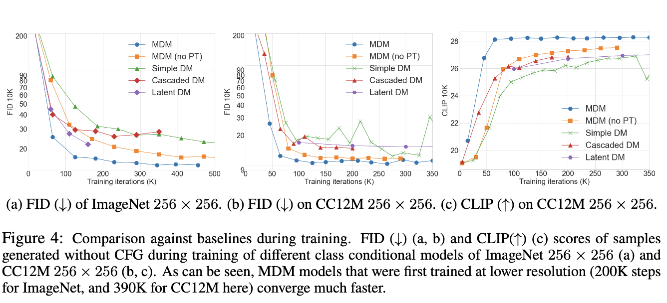
In conclusion, the introduction of Matryoshka Diffusion Models by researchers at Apple represents a significant step forward in high-resolution image and video generation. By leveraging a hierarchical structure and a progressive training schedule, MDM offers a more efficient and scalable solution than traditional methods. This advancement addresses the inefficiencies and complexities of existing diffusion models and paves the way for more practical and resource-efficient applications of AI-driven visual content creation. As a result, MDM holds great potential for future developments in the field, providing a robust framework for generating high-quality images and videos with reduced computational demands.
Check out the Paper and GitHub . All credit for this research goes to the researchers of this project. Also, don’t forget to follow us on Twitter and join our Telegram Channel and LinkedIn Gr oup . If you like our work, you will love our newsletter..
Don’t Forget to join our 48k+ ML SubReddit
Find Upcoming AI Webinars here
Arcee AI Released DistillKit: An Open Source, Easy-to-Use Tool Transforming Model Distillation for Creating Efficient, High-Performance Small Language Models

Nikhil is an intern consultant at Marktechpost. He is pursuing an integrated dual degree in Materials at the Indian Institute of Technology, Kharagpur. Nikhil is an AI/ML enthusiast who is always researching applications in fields like biomaterials and biomedical science. With a strong background in Material Science, he is exploring new advancements and creating opportunities to contribute.
InfinityMath: A Scalable Instruction Tuning Dataset for Programmatic Mathematical Reasoning
- ToolSandbox LLM Tool-Use Benchmark Released by Apple: A Conversational and Interactive Evaluation Benchmark for LLM Tool-Use Capabilities
- The AI Scientist: The World’s First AI System for Automating Scientific Research and Open-Ended Discovery
- Optimizing Spiking Neural P Systems Simulations: Achieving Unprecedented Speed and Efficiency through Compressed Matrix Representations on GPUs Using CUDA

RELATED ARTICLES MORE FROM AUTHOR
Prompt caching is now available on the anthropic api for specific claude models, xai released grok-2 beta: an ai model with unparalleled reasoning, benchmark-topping performance, and advanced capabilities, arcee ai introduces arcee swarm: a groundbreaking mixture of agents moa architecture inspired by the cooperative intelligence found in nature itself, linguistics-aware in-context learning with data augmentation (laida): an ai framework for enhanced metaphor components identification in nlp tasks, videollama 2 released: a set of video large language models designed to advance multimodal research in the arena of video-language modeling, arcee ai introduces arcee swarm: a groundbreaking mixture of agents moa architecture inspired by..., linguistics-aware in-context learning with data augmentation (laida): an ai framework for enhanced metaphor components..., videollama 2 released: a set of video large language models designed to advance multimodal..., meet david ai: the data marketplace for ai, harnessing ai for hormesis management and plant stress analysis: advancing agricultural resilience and productivity, toolsandbox llm tool-use benchmark released by apple: a conversational and interactive evaluation benchmark for..., llm for biology: this paper discusses how language models can be applied to biological....
- AI Magazine
- Privacy & TC
- Cookie Policy
- 🐝 Partnership and Promotion
Learn How To Curate Your AI Data At Scale [Webinar]
Thank You 🙌
Privacy Overview
Navigation Menu
Search code, repositories, users, issues, pull requests..., provide feedback.
We read every piece of feedback, and take your input very seriously.
Saved searches
Use saved searches to filter your results more quickly.
To see all available qualifiers, see our documentation .
- Notifications You must be signed in to change notification settings
[GGUF and Flux full fp16 Model] loading T5, CLIP + new VAE UI #1050
{{editor}}'s edit
Lllyasviel aug 13, 2024 maintainer.
| The old Automatic1111’s user interface of VAE selection is not powerful enough for modern models . Forge make minor modifications so that the UI is as close as possible to A1111 but also meet the demands of newer models.
Before:
After:
Before:
After:
Download base model and vae (raw float16) from Flux official and . Download clip-l and t5-xxl from or our Put base model in . Put vae in Put clip-l and t5 in You can load in nearly arbitrary combinations
etc ... Now you can even load clip-l for sd1.5 separately |
Beta Was this translation helpful? Give feedback.
Replies: 12 comments · 17 replies
Hmrmike aug 13, 2024.
| Boy is float16 Flux heavy! After some magical restarts, running fp16 without any Never OOM seems to work I like this way of handling VAE/encoders, but it feels like allowing to save some presets would be comfortable. It gets a bit tedious after switching models and might be confusing to less experienced users- forgetting CLIP or something will error out with "TypeError: 'NoneType' object is not iterable" on a checkpoint like fp16 Flux here, for example, and figuring it out is less trivial. We do have "You do not have CLIP state dict!" but it's buried in the traceback, almost invisible. Maybe a more obvious error message will be helpful at least. Well, fp8 so far seems most competent. For some reason fp16 messes up text more but the composition is nearly the same. nf4 deviates a lot is some cases. |
KSimulation Aug 15, 2024
| See |
| Which FP16 models you were using? |
HMRMike Aug 15, 2024
| This one linked in OP: |
Iory1998 Aug 15, 2024
| I have similar H/w to you but using the f16 version results in ForgeUI crashing. How did you manage to solve the OOM issue? |
| Lots of commits happened since that post, and maybe something was changed for memory management. Now I make sure these settings are set right after launching Forge, if the intent is to run fp16. Also haven't dared to try anything other than 1024x1024. |
ali0une Aug 13, 2024
| i think Forge Ui needs some dropdown menus like the ones i circled in red as they are choices and only one can be displayed when selected, that would help to take up less space on the screen : |
RamonGuthrie Aug 13, 2024
| Yeah I believe the VAE / Text Encoder when stacked, they should form a double row. Also a folder standard should be agreed on, forge is storing in and ComfyUI is storing these files in this will lead to doubling up models |
hollowstrawberry Aug 14, 2024
| I believe this broke the command line option. Also, could you add a option instead of hardcoding ? Thank you for all your work. |
evanheckert Aug 15, 2024
| Yes, and with --vae-dir set, the files in the forge text_encoder folder aren't detected either. |
abzaloff Aug 15, 2024
| Specify additionally --clip-models-path |
bews Aug 14, 2024
| Can't make it work for some reason on 4090: it shows the preview during the generation, but them doesn't give the final result. No errors in the console either. Meanwhile flux1-dev-fp8.safetensors works no problem. |
| Are you perhaps using TAESD instead of full VAE in the settings? |
bews Aug 15, 2024
| Nope
Edit: I tried resetting all settings and removing everything from the command line - nothing did help. |
Githb-alexsherman Aug 15, 2024
| How to open vae/text encoder I can't find it |
| Me too! It seems the T5, CLIP are not detected isn text_encoder folder |
ali0une Aug 15, 2024
| i only about this morning and it's already here in Forge ... also read this morning LoRA work now in nf4. Many thanks |
RamonGuthrie Aug 15, 2024
| Where did you read LoRAs working with nf4 models? |
supersonic13 Aug 15, 2024
| In this discussion: |
| , i've just tested i really don't know what to think, only the art_comfy_converted LoRA seems to produce an effect :-| Left is no LoRA, right is with _comfy_converted LoRA : woman taking a selfie art |
| i think the LoRA strength must be > 1, with 1.5 it clearly makes a difference. Left is no LoRA, right is with realism_comfy_converted LoRA : woman taking a selfie |
yamfun Aug 15, 2024
| does the clip and vae path respect the args --vae-dir and --clip-models-path?? seems no... |
jepjoo Aug 15, 2024
| Did not work for me. I resorted to using symbolic links (in Windows). Also the fact that Forge wants checkpoint and unet files in the same folder but ComfyUI separates them into two different ones is slightly cumbersome as I use ComfyUI installation for storing all the actual model files. |
ishadowx27 Aug 15, 2024
| This is why I use StabilityMatrix since it manages everything, including the downloading of models from different sites. |
tazztone Aug 15, 2024
| now would be great if the XYZ grid function was working to make comparisons :) |
rabidcopy Aug 15, 2024
| GGUF Q4_0 inference speed is faster than FP8 for me, though unfortunately it takes 100+ seconds to move the model/transformer each time, making the speed increase moot as a minimum of 100 seconds is added to each generation. Dunno why, when loading a FP8 Flux model, model moving for CLIP+T5/Transformer/VAE are all ~0 seconds. When introducing the Q4_0 quantization of the transformer, it takes 100-300 seconds to move the mode/transformer and begin inference. This is without Loras. I'm going to assume part of the reason is being on a low VRAM/RAM system and relying on a swap file. Though I figured loading an even smaller transformer would of been less prone to RAM/Swap related issues. |
| Has someone done a video about GGUF quants with Flux? Is it because this stuff is moving too fast? |
| I have an RTX3090 and 32GB of ram. ForgeUI crashes when I try to use the fp16 and I see in console the message "Using Default T5 Data Type: torch.float16". I can use the full precision in ComfyUI without a hitch. |
- Numbered list
- Unordered list
- Attach files
Select a reply
Information
- Author Services
Initiatives
You are accessing a machine-readable page. In order to be human-readable, please install an RSS reader.
All articles published by MDPI are made immediately available worldwide under an open access license. No special permission is required to reuse all or part of the article published by MDPI, including figures and tables. For articles published under an open access Creative Common CC BY license, any part of the article may be reused without permission provided that the original article is clearly cited. For more information, please refer to https://www.mdpi.com/openaccess .
Feature papers represent the most advanced research with significant potential for high impact in the field. A Feature Paper should be a substantial original Article that involves several techniques or approaches, provides an outlook for future research directions and describes possible research applications.
Feature papers are submitted upon individual invitation or recommendation by the scientific editors and must receive positive feedback from the reviewers.
Editor’s Choice articles are based on recommendations by the scientific editors of MDPI journals from around the world. Editors select a small number of articles recently published in the journal that they believe will be particularly interesting to readers, or important in the respective research area. The aim is to provide a snapshot of some of the most exciting work published in the various research areas of the journal.
Original Submission Date Received: .
- Active Journals
- Find a Journal
- Proceedings Series
- For Authors
- For Reviewers
- For Editors
- For Librarians
- For Publishers
- For Societies
- For Conference Organizers
- Open Access Policy
- Institutional Open Access Program
- Special Issues Guidelines
- Editorial Process
- Research and Publication Ethics
- Article Processing Charges
- Testimonials
- Preprints.org
- SciProfiles
- Encyclopedia
Article Menu

- Subscribe SciFeed
- Recommended Articles
- Google Scholar
- on Google Scholar
- Table of Contents
Find support for a specific problem in the support section of our website.
Please let us know what you think of our products and services.
Visit our dedicated information section to learn more about MDPI.
JSmol Viewer
When games influence words: gaming addiction among college students increases verbal aggression through risk-biased drifting in decision-making.

1. Introduction
1.1. game addiction and game violence, 1.2. verbal aggression, 1.3. inhibitory control, 1.4. risk preference, 1.5. mediation model, 1.6. the present study, 2.1. participants, 2.2. research instruments, 2.2.1. questionnaires, 2.2.2. antisaccade task, 2.2.3. go/no-go task, 2.2.4. the cup task, 2.3. procedure, 2.4. statistical analysis, 2.4.1. validity analysis, 2.4.2. the hierarchical drift diffusion model, 2.4.3. mediation model, 3.1. correlational analysis and the cut-off point for gaming addiction, 3.2. validity analysis, 3.3. hierarchical drift diffusion model, 3.4. mediation model, 4. discussion, 4.1. mediation model, 4.2. risk preference, 4.3. inhibitory control, 4.4. contribution of the present study, 4.5. limitations, 5. conclusions, supplementary materials, author contributions, institutional review board statement, informed consent statement, data availability statement, conflicts of interest.
- Statista. Number of Video Gamers Worldwide in 2021, by Region. 2022. Available online: https://www.statista.com/statistics/293304/number-video-gamers/#:~:text=Figures%20in%202020%20showed%20that,across%20the%20globe%20in%202020 (accessed on 23 October 2023).
- Statista. Number of Video Gamers in the United States in 2022, by Engagement Level. 2022. Available online: https://www.statista.com/statistics/300942/number-core-gamers-usa/ (accessed on 23 October 2023).
- Bickham, D.S. Current Research and Viewpoints on Internet Addiction in Adolescents. Curr. Pediatr. Rep. 2021 , 9 , 1–10. [ Google Scholar ] [ CrossRef ] [ PubMed ]
- Chen, Y.-Y.; Yim, H.; Lee, T.-H. Negative Impact of Daily Screen Use on Inhibitory Control Network in Preadolescence: A Two-Year Follow-up Study. Dev. Cogn. Neurosci. 2023 , 60 , 101218. [ Google Scholar ] [ CrossRef ] [ PubMed ]
- Lin, H.-P.; Chen, K.-L.; Chou, W.; Yuan, K.-S.; Yen, S.-Y.; Chen, Y.-S.; Chow, J.C. Prolonged Touch Screen Device Usage Is Associated with Emotional and Behavioral Problems, but Not Language Delay, in Toddlers. Infant Behav. Dev. 2020 , 58 , 101424. [ Google Scholar ] [ CrossRef ] [ PubMed ]
- Wiederhold, B.K. Kids Will Find a Way: The Benefits of Social Video Games. Cyberpsychology Behav. Soc. Netw. 2021 , 24 , 213–214. [ Google Scholar ] [ CrossRef ]
- Sokolov, A.A.; Collignon, A.; Bieler-Aeschlimann, M. Serious Video Games and Virtual Reality for Prevention and Neurorehabilitation of Cognitive Decline Because of Aging and Neurodegeneration. Curr. Opin. Neurol. 2020 , 33 , 239–248. [ Google Scholar ] [ CrossRef ]
- Anderson, C.A.; Bushman, B.J. Human Aggression. Annu. Rev. Psychol. 2001 , 52 , 27–51. [ Google Scholar ] [ CrossRef ]
- Buckley, K.E.; Anderson, C.A. A Theoretical Model of the Effects and Consequences of Playing Video Games. In Playing Video Games: Motives, Responses, and Consequences ; Vorderer, P., Bryant, J., Eds.; Lawrence Erlbaum Associates Publishers: Mahwah, NJ, USA, 2006; pp. 363–378. [ Google Scholar ]
- Drummond, A.; Sauer, J.D.; Ferguson, C.J. Do Longitudinal Studies Support Long-Term Relationships between Aggressive Game Play and Youth Aggressive Behaviour? A Meta-Analytic Examination. R. Soc. Open Sci. 2020 , 7 , 200373. [ Google Scholar ] [ CrossRef ]
- Mariano, T.E.; Gouveia, V.V.; Pimentel, C.E. The Effect of Video Games on Positive and Negative Cognitions. RPI 2020 , 12 , 7. [ Google Scholar ] [ CrossRef ]
- Shoshani, A.; Braverman, S.; Meirow, G. Video Games and Close Relations: Attachment and Empathy as Predictors of Children’s and Adolescents’ Video Game Social Play and Socio-Emotional Functioning. Comput. Hum. Behav. 2021 , 114 , 106578. [ Google Scholar ] [ CrossRef ]
- Tian, Y.; Gao, M.; Wang, P.; Gao, F. The Effects of Violent Video Games and Shyness on Individuals’ Aggressive Behaviors. Aggress. Behav. 2020 , 46 , 16–24. [ Google Scholar ] [ CrossRef ]
- Lee, E.-J.; Kim, H.S.; Choi, S. Violent Video Games and Aggression: Stimulation or Catharsis or Both? Cyberpsychology Behav. Soc. Netw. 2021 , 24 , 41–47. [ Google Scholar ] [ CrossRef ] [ PubMed ]
- Weber, R.; Behr, K.M.; Fisher, J.T.; Lonergan, C.; Quebral, C. Video Game Violence and Interactivity: Effect or Equivalence? J. Commun. 2020 , 70 , 219–244. [ Google Scholar ] [ CrossRef ]
- Li, S.; Wu, Z.; Zhang, Y.; Xu, M.; Wang, X.; Ma, X. Internet Gaming Disorder and Aggression: A Meta-Analysis of Teenagers and Young Adults. Front. Public Health 2023 , 11 , 1111889. [ Google Scholar ] [ CrossRef ] [ PubMed ]
- Zhang, Q.; Cao, Y.; Tian, J. Effects of violent video games on players’ and observers’ aggressive cognitions and aggressive behaviors. J. Exp. Child Psychol. 2021 , 203 , 105005. [ Google Scholar ] [ CrossRef ] [ PubMed ]
- Khoo, S.S.; Yang, H. Smartphone Addiction and Checking Behaviors Predict Aggression: A Structural Equation Modeling Approach. IJERPH 2021 , 18 , 13020. [ Google Scholar ] [ CrossRef ]
- Addo, P.C.; Fang, J.; Kulbo, N.B.; Gumah, B.; Dagadu, J.C.; Li, L. Violent Video Games and Aggression Among Young Adults: The Moderating Effects of Adverse Environmental Factors. Cyberpsychology Behav. Soc. Netw. 2021 , 24 , 17–23. [ Google Scholar ] [ CrossRef ]
- Peng, C.; Guo, T.; Cheng, J.; Wang, M.; Rong, F.; Zhang, S.; Tan, Y.; Ding, H.; Wang, Y.; Yu, Y. Sex Differences in Association between Internet Addiction and Aggression among Adolescents Aged 12 to 18 in Mainland of China. J. Affect. Disord. 2022 , 312 , 198–207. [ Google Scholar ] [ CrossRef ]
- American Psychiatric Association. Diagnostic and Statistical Manual of Mental Disorders , 5th ed.; American Psychiatric Publishing: Arlington, VA, USA, 2013. [ Google Scholar ] [ CrossRef ]
- Anderson, C.A.; Bushman, B.J.; Bartholow, B.D.; Cantor, J.; Christakis, D.; Coyne, S.M.; Donnerstein, E.; Brockmyer, J.F.; Gentile, D.A.; Green, C.S.; et al. Screen Violence and Youth Behavior. Pediatrics 2017 , 140 (Suppl. 2), S142–S147. [ Google Scholar ] [ CrossRef ]
- Király, O.; Sleczka, P.; Pontes, H.M.; Urbán, R.; Griffiths, M.D.; Demetrovics, Z. Validation of the Ten-Item Internet Gaming Disorder Test (IGDT-10) and evaluation of the nine DSM-5 Internet Gaming Disorder criteria. Addict. Behav. 2017 , 64 , 253–260. [ Google Scholar ] [ CrossRef ]
- Mohammad, S.; Jan, R.A.; Alsaedi, S.L. Symptoms, Mechanisms, and Treatments of Video Game Addiction. Cureus 2023 , 15 , e36957. [ Google Scholar ] [ CrossRef ]
- Mihara, S.; Higuchi, S. Cross-sectional and longitudinal epidemiological studies of Internet gaming disorder: A systematic review of the literature. Psychiatry Clin. Neurosci. 2017 , 71 , 425–444. [ Google Scholar ] [ CrossRef ] [ PubMed ]
- Adachi, P.J.; Willoughby, T. The Longitudinal Association between Competitive Video Game Play and Aggression among Adolescents and Young Adults. Child Dev. 2016 , 87 , 1877–1892. [ Google Scholar ] [ CrossRef ] [ PubMed ]
- Wang, L.; Yang, G.; Zheng, Y.; Li, Z.; Qi, Y.; Li, Q.; Liu, X. Enhanced neural responses in specific phases of reward processing in individuals with Internet gaming disorder. J. Behav. Addict. 2021 , 10 , 99–111. [ Google Scholar ] [ CrossRef ] [ PubMed ]
- Fuji, K.; Yoshida, F. The influences of interaction during online gaming on sociability and aggression in real life. Shinrigaku Kenkyu Jpn. J. Psychol. 2010 , 80 , 494–503. [ Google Scholar ] [ CrossRef ] [ PubMed ]
- Ducharme, P.; Kahn, J.; Vaudreuil, C.; Gusman, M.; Waber, D.; Ross, A.; Rotenberg, A.; Rober, A.; Kimball, K.; Peechatka, A.L.; et al. A “Proof of Concept” Randomized Controlled Trial of a Video Game Requiring Emotional Regulation to Augment Anger Control Training. Front. Psychiatry 2021 , 12 , 591906. [ Google Scholar ] [ CrossRef ] [ PubMed ]
- Chen, S.; Wei, M.; Wang, X.; Liao, J.; Li, J.; Liu, Y. Competitive Video Game Exposure Increases Aggression through Impulsivity in Chinese Adolescents: Evidence from a Multi-Method Study. J. Youth Adolesc. 2024; advance online publication . [ Google Scholar ] [ CrossRef ]
- Wei, L.; Zhang, S.; Turel, O.; Bechara, A.; He, Q. A Tripartite Neurocognitive Model of Internet Gaming Disorder. Front. Psychiatry 2017 , 8 , 285. [ Google Scholar ] [ CrossRef ] [ PubMed ]
- Gong, Y.; Li, Q.; Li, J.; Wang, X.; Jiang, W.; Zhao, W. Does Early Adversity Predict Aggression Among Chinese Male Violent Juvenile Offenders? The Mediating Role of Life History Strategy and the Moderating Role of Meaning in Life. BMC Psychol. 2023 , 11 , 382. [ Google Scholar ] [ CrossRef ]
- Glascock, J. Contribution of Verbally Aggressive TV Exposure and Perceived Reality to Trait Verbal Aggression. Commun. Rep. 2021 , 34 , 151–164. [ Google Scholar ] [ CrossRef ]
- McCarthy, B.; Boland, A.; Murphy, S.; Cooney, C. Vocally Disruptive Behavior: A Case Report and Literature Review. Ir. J. Psychol. Med. 2022 , 39 , 97–102. [ Google Scholar ] [ CrossRef ]
- Poling, D.V.; Smith, S.W. Perceptions about Verbal Aggression: Survey of Secondary Students with Emotional and Behavioral Disorders. J. Emot. Behav. Disord. 2023 , 31 , 14–26. [ Google Scholar ] [ CrossRef ]
- Infante, D.A.; Chandler, T.A.; Rudd, J.E. Test of an Argumentative Skill Deficiency Model of Interpersonal Violence. Commun. Monogr. 1989 , 56 , 163–177. [ Google Scholar ] [ CrossRef ]
- Joshi, A.; Sharma, K.; Sigdel, D.; Thapa, T.; Mehta, R. Internet Gaming Disorder and Aggression among Students on School Closure during COVID-19 Pandemic. J. Nepal Health Res. Counc. 2022 , 20 , 41–46. [ Google Scholar ] [ CrossRef ] [ PubMed ]
- Columb, D.; Wong, M.C.; O’Mahony, V.; Harrington, C.; Griffiths, M.D.; O’Gara, C. Gambling Advertising during Live Televised Male Sporting Events in Ireland: A Descriptive Study. Ir. J. Psychol. Med. 2023 , 40 , 134–142. [ Google Scholar ] [ CrossRef ]
- McNamee, P.; Mendolia, S.; Yerokhin, O. Social Media Use and Emotional and Behavioural Outcomes in Adolescence: Evidence from British Longitudinal Data. Econ. Hum. Biol. 2021 , 41 , 100992. [ Google Scholar ] [ CrossRef ] [ PubMed ]
- Parrish, K.H.; Smith, M.R.; Moran, L.; Ruberry, E.J.; Lengua, L.J. Tests of Bidirectional Relations of TV Exposure and Effortful Control as Predictors of Adjustment in Early Childhood in the Context of Family Risk Factors. Infant Child Dev. 2022 , 31 , e2314. [ Google Scholar ] [ CrossRef ]
- Limtrakul, N.; Louthrenoo, O.; Narkpongphun, A.; Boonchooduang, N.; Chonchaiya, W. Media Use and Psychosocial Adjustment in Children and Adolescents. J. Paediatr. Child Health 2018 , 54 , 296–301. [ Google Scholar ] [ CrossRef ] [ PubMed ]
- Varghese, N.E.; Santoro, E.; Lugo, A.; Madrid-Valero, J.J.; Ghislandi, S.; Torbica, A.; Gallus, S. The Role of Technology and Social Media Use in Sleep-Onset Difficulties among Italian Adolescents: Cross-sectional Study. J. Med. Internet Res. 2021 , 23 , e20319. [ Google Scholar ] [ CrossRef ] [ PubMed ]
- Brand, M.; Wegmann, E.; Stark, R.; Müller, A.; Wölfling, K.; Robbins, T.W.; Potenza, M.N. The Interaction of Person-Affect-Cognition-Execution (I-PACE) Model for Addictive Behaviors: Update, Generalization to Addictive Behaviors beyond Internet-Use Disorders, and Specification of the Process Character of Addictive Behaviors. Neurosci. Biobehav. Rev. 2019 , 104 , 1–10. [ Google Scholar ] [ CrossRef ] [ PubMed ]
- Argyriou, E.; Davison, C.B.; Lee, T.T.C. Response Inhibition and Internet Gaming Disorder: A Meta-analysis. Addict. Behav. 2017 , 71 , 54–60. [ Google Scholar ] [ CrossRef ]
- Bounoua, N.; Spielberg, J.M.; Sadeh, N. Clarifying the Synergistic Effects of Emotion Dysregulation and Inhibitory Control on Physical Aggression. Hum. Brain Mapp. 2022 , 43 , 5358–5369. [ Google Scholar ] [ CrossRef ]
- Dong, G.-H.; Potenza, M.N. Considering Gender Differences in the Study and Treatment of Internet Gaming Disorder. J. Psychiatr. Res. 2022 , 153 , 25–29. [ Google Scholar ] [ CrossRef ] [ PubMed ]
- Qiu, B.; Chen, Y.; He, X.; Liu, T.; Wang, S.; Zhang, W. Short-Term Touch-Screen Video Game Playing Improves the Inhibition Ability. Int. J. Environ. Res. Public Health 2021 , 18 , 6884. [ Google Scholar ] [ CrossRef ]
- Goldstein, R.; Volkow, N. Dysfunction of the prefrontal cortex in addiction: Neuroimaging findings and clinical implications. Nat. Rev. Neurosci. 2011 , 12 , 652–669. [ Google Scholar ] [ CrossRef ]
- Everitt, B.J.; Robbins, T.W. Drug Addiction: Updating Actions to Habits to Compulsions Ten Years On. Annu. Rev. Psychol. 2016 , 67 , 23–50. [ Google Scholar ] [ CrossRef ]
- Amlung, M.; Vedelago, L.; Acker, J.; Balodis, I.; MacKillop, J. Steep delay discounting and addictive behavior: A meta-analysis of continuous associations. Addiction 2017 , 112 , 51–62. [ Google Scholar ] [ CrossRef ]
- Turel, O.; He, Q.; Brevers, D.; Bechara, A. Delay discounting mediates the association between posterior insular cortex volume and social media addiction symptoms. Cogn. Affect. Behav. Neurosci. 2018 , 18 , 694–704. [ Google Scholar ] [ CrossRef ] [ PubMed ]
- Verdejo-Garcia, A.; Pérez-García, M.; Bechara, A. Emotion, decision-making and substance dependence: A somatic-marker model of addiction. Curr. Neuropharmacol. 2006 , 4 , 17–31. [ Google Scholar ] [ CrossRef ] [ PubMed ]
- Noh, D.; Shim, M.S. Factors influencing smartphone overdependence among adolescents. Sci. Rep. 2024 , 14 , 7725. [ Google Scholar ] [ CrossRef ] [ PubMed ]
- Wang, H.; Xu, S.; Wang, S.; Wang, Y.; Chen, R. Using decision tree to predict non-suicidal self-injury among young adults: The role of depression, childhood maltreatment and recent bullying victimization. Eur. J. Psychotraumatol. 2024 , 15 , 2322390. [ Google Scholar ] [ CrossRef ] [ PubMed ]
- Dooren, M.M.M.V.; Visch, V.T.; Spijkerman, R. The Design and Application of Game Rewards in Youth Addiction Care. Information 2019 , 10 , 126. [ Google Scholar ] [ CrossRef ]
- Zheng, Y.; He, J.; Fan, L.; Qiu, Y. Reduction of Symptom after a Combined Behavioral Intervention for Reward Sensitivity and Rash Impulsiveness in Internet Gaming Disorder: A Comparative Study. J. Psychiatr. Res. 2022 , 153 , 159–166. [ Google Scholar ] [ CrossRef ] [ PubMed ]
- Dell’Osso, B.; Di Bernardo, I.; Vismara, M.; Piccoli, E.; Giorgetti, F.; Molteni, L.; Fineberg, N.A.; Virzì, C.; Bowden-Jones, H.; Truzoli, R.; et al. Managing Problematic Usage of the Internet and Related Disorders in an Era of Diagnostic Transition: An Updated Review. CPEMH 2021 , 17 , 61–74. [ Google Scholar ] [ CrossRef ] [ PubMed ]
- Müller, S.M.; Antons, S.; Wegmann, E.; Ioannidis, K.; King, D.L.; Potenza, M.N.; Chamberlain, S.R.; Brand, M. A Systematic Review and Meta-analysis of Risky Decision-making in Specific Domains of Problematic Use of the Internet: Evidence across Different Decision-making Tasks. Neurosci. Biobehav. Rev. 2023 , 152 , 105271. [ Google Scholar ] [ CrossRef ] [ PubMed ]
- Kim, Y.-J.; Lim, J.A.; Lee, J.Y.; Oh, S.; Kim, S.N.; Kim, D.J.; Ha, J.E.; Kwon, J.S.; Choi, J.-S. Impulsivity and Compulsivity in Internet Gaming Disorder: A Comparison with Obsessive–Compulsive Disorder and Alcohol Use Disorder. J. Behav. Addict. 2017 , 6 , 545–553. [ Google Scholar ] [ CrossRef ] [ PubMed ]
- Kräplin, A.; Scherbaum, S.; Kraft, E.-M.; Rehbein, F.; Bühringer, G.; Goschke, T.; Mößle, T. The Role of Inhibitory Control and Decision-making in the Course of Internet Gaming Disorder. J. Behav. Addict. 2021 , 9 , 990–1001. [ Google Scholar ] [ CrossRef ]
- Vega, A.; Cabello, R.; Megías-Robles, A.; Gómez-Leal, R.; Fernández-Berrocal, P. Emotional Intelligence and Aggressive Behaviors in Adolescents: A Systematic Review and Meta-Analysis. Trauma Violence Abus. 2022 , 23 , 1173–1183. [ Google Scholar ] [ CrossRef ] [ PubMed ]
- Yan, W.S.; Chen, R.T.; Liu, M.M.; Zheng, D.H. Monetary Reward Discounting, Inhibitory Control, and Trait Impulsivity in Young Adults with Internet Gaming Disorder and Nicotine Dependence. Front. Psychiatry 2021 , 12 , 628933. [ Google Scholar ] [ CrossRef ] [ PubMed ]
- Noël, X.; Brevers, D.; Bechara, A. A neurocognitive approach to understanding the neurobiology of addiction. Curr. Opin. Neurobiol. 2013 , 23 , 632–638. [ Google Scholar ] [ CrossRef ]
- Lin, Y.; Feng, T. Lateralization of self-control over the dorsolateral prefrontal cortex in decision-making: A systematic review and meta-analytic evidence from noninvasive brain stimulation. Cogn. Affect. Behav. Neurosci. 2024 , 24 , 19–41. [ Google Scholar ] [ CrossRef ]
- Laino Chiavegatti, G.; Floresco, S.B. Acute stress differentially alters reward-related decision making and inhibitory control under threat of punishment. Neurobiol. Stress 2024 , 30 , 100633. [ Google Scholar ] [ CrossRef ]
- Pontes, H.M.; Király, O.; Demetrovics, Z.; Griffiths, M.D. The Conceptualisation and Measurement of DSM-5 Internet Gaming Disorder: The Development of the IGD-20 Test. PLoS ONE 2014 , 9 , e110137. [ Google Scholar ] [ CrossRef ] [ PubMed ]
- Carlo, G.; Randall, B.A. The Development of a Measure of Prosocial Behaviors for Late Adolescents. J. Youth Adolesc. 2002 , 31 , 31–44. [ Google Scholar ] [ CrossRef ]
- Buss, A.H.; Perry, M. Personality Processes and Individual Differences. J. Pers. Soc. Psychol. 1992 , 63 , 452–459. [ Google Scholar ] [ CrossRef ] [ PubMed ]
- Miyake, A.; Friedman, N.P.; Emerson, M.J.; Witzki, A.H.; Howerter, A.; Wager, T.D. The Unity and Diversity of Executive Functions and Their Contributions to Complex “Frontal Lobe” Tasks: A Latent Variable Analysis. Cogn. Psychol. 2000 , 41 , 49–100. [ Google Scholar ] [ CrossRef ] [ PubMed ]
- Nosek, B.A.; Greenwald, A.G.; Banaji, M.R. Understanding and Using the Implicit Association Test: II. Method Variables and Construct Validity. Pers. Soc. Psychol. Bull. 2005 , 31 , 166–180. [ Google Scholar ] [ CrossRef ] [ PubMed ]
- Levin, I.P.; Hart, S.S. Risk Preferences in Young Children: Early Evidence of Individual Differences in Reaction to Potential Gains and Losses. J. Behav. Decis. Mak. 2003 , 16 , 397–413. [ Google Scholar ] [ CrossRef ]
- Gelman, A.; Rubin, D.B. Markov Chain Monte Carlo Methods in Biostatistics. Stat. Methods Med. Res. 1996 , 5 , 339–355. [ Google Scholar ] [ CrossRef ]
- Saleh, Y.; Jarratt-Barnham, I.; Petitet, P.; Fernandez-Egea, E.; Manohar, S.G.; Husain, M. Negative symptoms and cognitive impairment are associated with distinct motivational deficits in treatment resistant schizophrenia. Mol. Psychiatry 2023 , 28 , 4831–4841. [ Google Scholar ] [ CrossRef ]
- Jun, W. A Study on the Cause Analysis of Cyberbullying in Korean Adolescents. Int. J. Environ. Res. Public Health 2020 , 17 , 4648. [ Google Scholar ] [ CrossRef ]
- She, Y.; Yang, Z.; Xu, L.; Li, L. The Association between Violent Video Game Exposure and Sub-Types of School Bullying in Chinese Adolescents. Front. Psychiatry 2022 , 13 , 1026625. [ Google Scholar ] [ CrossRef ]
- Johnson, E.P.; Samp, J.A. Stoicism and Verbal Aggression in Serial Arguments: The Roles of Perceived Power, Perceived Resolvability, and Frequency of Arguments. J. Interpers. Violence 2022 , 37 , NP11836–NP11856. [ Google Scholar ] [ CrossRef ] [ PubMed ]
- Dong, G.; Huang, J.; Du, X. Enhanced reward sensitivity and decreased loss sensitivity in Internet addicts: An fMRI study during a guessing task. J. Psychiatr. Res. 2011 , 45 , 1525–1529. [ Google Scholar ] [ CrossRef ] [ PubMed ]
- Byrd, A.L.; Hawes, S.W.; Waller, R.; Delgado, M.R.; Sutherland, M.T.; Dick, A.S.; Trucco, E.M.; Riedel, M.C.; Pacheco-Colón, I.; Laird, A.R.; et al. Neural response to monetary loss among youth with disruptive behavior disorders and callous-unemotional traits in the ABCD study. NeuroImage Clin. 2021 , 32 , 102810. [ Google Scholar ] [ CrossRef ] [ PubMed ]
- Wang, L.; Tian, M.; Zheng, Y.; Li, Q.; Liu, X. Reduced Loss Aversion and Inhibitory Control in Adolescents with Internet Gaming Disorder. Psychol. Addict. Behav. 2020 , 34 , 484–496. [ Google Scholar ] [ CrossRef ] [ PubMed ]
- Bediou, B.; Adams, D.M.; Mayer, R.E.; Tipton, E.; Green, C.S.; Bavelier, D. Meta-Analysis of Action Video Game Impact on Perceptual, Attentional, and Cognitive Skills. Psychol. Bull. 2018 , 144 , 77–110. [ Google Scholar ] [ CrossRef ] [ PubMed ]
- Pichon, S.; Bediou, B.; Antico, L.; Jack, R.; Garrod, O.; Sims, C.; Green, C.S.; Schyns, P.; Bavelier, D. Emotion perception in habitual players of action video games. Emotion 2021 , 21 , 1324–1339. [ Google Scholar ] [ CrossRef ]
- Foland-Ross, L.C.; Buckingam, B.; Mauras, N.; Arbelaez, A.M.; Tamborlane, W.V.; Tsalikian, E.; Cato, A.; Tong, G.; Englert, K.; Mazaika, P.K.; et al. Diabetes Research in Children Network (DirecNet). Executive task-based brain function in children with type 1 diabetes: An observational study. PLoS Med. 2019 , 16 , e1002979. [ Google Scholar ] [ CrossRef ]
- Lamp, G.; Sola Molina, R.M.; Hugrass, L.; Beaton, R.; Crewther, D.; Crewther, S.G. Kinematic Studies of the Go/No-Go Task as a Dynamic Sensorimotor Inhibition Task for Assessment of Motor and Executive Function in Stroke Patients: An Exploratory Study in a Neurotypical Sample. Brain Sci. 2022 , 12 , 1581. [ Google Scholar ] [ CrossRef ]
- Cabedo-Peris, J.; González-Sala, F.; Merino-Soto, C.; Pablo, J.Á.C.; Toledano-Toledano, F. Decision Making in Addictive Behaviors Based on Prospect Theory: A Systematic Review. Healthcare 2022 , 10 , 1659. [ Google Scholar ] [ CrossRef ]
- Schiebener, J.; Zamarian, L.; Delazer, M.; Brand, M. Executive functions, categorization of probabilities, and learning from feedback: What does really matter for decision making under explicit risk conditions? J. Clin. Exp. Neuropsychol. 2011 , 33 , 1025–1039. [ Google Scholar ] [ CrossRef ]
- Toplak, M.E.; Sorge, G.B.; Benoit, A.; West, R.F.; Stanovich, K.E. Decision-making and cognitive abilities: A review of associations between Iowa Gambling Task performance, executive functions, and intelligence. Clin. Psychol. Rev. 2010 , 30 , 562–581. [ Google Scholar ] [ CrossRef ] [ PubMed ]
- Stover, A.D.; Shulkin, J.; Lac, A.; Rapp, T. A meta-analysis of cognitive reappraisal and personal resilience. Clin. Psychol. Rev. 2024 , 110 , 102428. [ Google Scholar ] [ CrossRef ]
- Etxandi, M.; Baenas, I.; Mora-Maltas, B.; Granero, R.; Fernández-Aranda, F.; Tovar, S.; Solé-Morata, N.; Lucas, I.; Casado, S.; Gómez-Peña, M.; et al. Are Signals Regulating Energy Homeostasis Related to Neuropsychological and Clinical Features of Gambling Disorder? A Case-Control Study. Nutrients 2022 , 14 , 5084. [ Google Scholar ] [ CrossRef ] [ PubMed ]
- Riek, H.C.; Brien, D.C.; Coe, B.C.; Huang, J.; Perkins, J.E.; Yep, R.; McLaughlin, P.M.; Orange, J.B.; Peltsch, A.J.; Roberts, A.C.; et al. Cognitive correlates of antisaccade behaviour across multiple neurodegenerative diseases. Brain Commun. 2023 , 5 , fcad049. [ Google Scholar ] [ CrossRef ]
- Johansson, M.E.; Cameron, I.G.M.; Van der Kolk, N.M.; de Vries, N.M.; Klimars, E.; Toni, I.; Bloem, B.R.; Helmich, R.C. Aerobic Exercise Alters Brain Function and Structure in Parkinson’s Disease: A Randomized Controlled Trial. Ann. Neurol. 2022 , 91 , 203–216. [ Google Scholar ] [ CrossRef ] [ PubMed ]
- Magee, K.E.; McClaine, R.; Laurianti, V.; Connell, A.M. Effects of binge drinking and depression on cognitive-control processes during an emotional Go/No-Go task in emerging adults. J. Psychiatr. Res. 2023 , 162 , 161–169. [ Google Scholar ] [ CrossRef ] [ PubMed ]
- Reed, P. Impact of Social Media Use on Executive Function. Comput. Hum. Behav. 2023 , 141 , 107598. [ Google Scholar ] [ CrossRef ]
- Gao, Q.; Jia, G.; Zhao, J.; Zhang, D. Inhibitory Control in Excessive Social Networking Users: Evidence From an Event-Related Potential-Based Go-Nogo Task. Front. Psychol. 2019 , 10 , 1810. [ Google Scholar ] [ CrossRef ]
- Casey, B.J.; Jones, R.M.; Hare, T.A. The Adolescent Brain. Ann. N. Y. Acad. Sci. 2008 , 1124 , 111–126. [ Google Scholar ] [ CrossRef ]
- Galvan, A.; Hare, T.A.; Parra, C.E.; Penn, J.; Voss, H.; Glover, G.; Casey, B.J. Earlier Development of the Accumbens Relative to Orbitofrontal Cortex Might Underlie Risk-Taking Behavior in Adolescents. J. Neurosci. 2006 , 26 , 6885–6892. [ Google Scholar ] [ CrossRef ]
- Galvan, A.; Hare, T.; Voss, H.; Glover, G.; Casey, B. Risk-Taking and the Adolescent Brain: Who Is at Risk? Dev. Sci. 2007 , 10 , F8–F14. [ Google Scholar ] [ CrossRef ] [ PubMed ]
- Grace, A.A.; Floresco, S.B.; Goto, Y.; Lodge, D.J. Regulation of Firing of Dopaminergic Neurons and Control of Goal-Directed Behaviors. Trends Neurosci. 2007 , 30 , 220–227. [ Google Scholar ] [ CrossRef ] [ PubMed ]
- Larche, C.J.; Chini, K.; Lee, C.; Dixon, M.J. To Pay or Just Play? Examining Individual Differences Between Purchasers and Earners of Loot Boxes in Overwatch. J. Gambl. Stud. 2023 , 39 , 625–643. [ Google Scholar ] [ CrossRef ] [ PubMed ]
- Zendle, D.; Flick, C.; Halgarth, D.; Ballou, N.; Cutting, J.; Drachen, A. The Relationship Between Lockdowns and Video Game Playtime: Multilevel Time-Series Analysis Using Massive-Scale Data Telemetry. J. Med. Internet Res. 2023 , 25 , e40190. [ Google Scholar ] [ CrossRef ] [ PubMed ]
- Lindenberg, K.; Holtmann, M. Einzug der Computerspielstörung als Verhaltenssucht in die ICD-11. Z. Kinder-Jugendpsychiatr. Psychother. 2022 , 50 , 1–7. [ Google Scholar ] [ CrossRef ] [ PubMed ]
- Lindenberg, K.; Kindt, S.; Szász-Janocha, C. Effectiveness of Cognitive Behavioral Therapy–Based Intervention in Preventing Gaming Disorder and Unspecified Internet Use Disorder in Adolescents: A Cluster Randomized Clinical Trial. JAMA Netw. Open 2022 , 5 , e2148995. [ Google Scholar ] [ CrossRef ] [ PubMed ]
- Zack, M.; St. George, R.; Clark, L. Dopaminergic signaling of uncertainty and the aetiology of gambling addiction. Prog. Neuro-Psychopharmacol. Biol. Psychiatry 2020 , 99 , 109853. [ Google Scholar ] [ CrossRef ]
- Dong, G.H.; Dai, J.; Potenza, M.N. Ten years of research on the treatments of internet gaming disorder: A scoping review and directions for future research. J. Behav. Addict. 2024 , 13 , 51–65. [ Google Scholar ] [ CrossRef ]
- Qin, L.; Liu, Q.; Luo, T. Reliability and Validity of the Chinese Version of the Internet Gaming Disorder Scale among College Students. Chin. J. Clin. Psychol. 2020 , 28 , 33–36. [ Google Scholar ] [ CrossRef ]
- Kou, Y.; Hong, H.; Tan, C.; Li, L. Revision of the Prosocial Tendency Scale for Adolescents. Psychol. Dev. Educ. 2007 , 1 , 112–117. [ Google Scholar ]
- Li, X.; Fei, L.; Zhang, Y.; Niu, Y.; Tong, Y.; Yang, S. Revision and Reliability and Validity of the Chinese Version of the Buss and Perry Aggression Questionnaire. Chin. J. Neurol. Psychiatr. 2011 , 10 , 607–613. [ Google Scholar ]
Click here to enlarge figure
| Recreation Program | M | SD |
|---|---|---|
| Video game | 59.29 | 70.77 |
| TV | 40.96 | 48.10 |
| Short video | 78.02 | 72.62 |
| Card game | 4.61 | 17.68 |
| Text-based media | 38.77 | 48.52 |
| Webcast | 7.00 | 25.30 |
| Terms | Explanations |
|---|---|
| a | The threshold in the risk advantage condition when winning money is used as feedback. |
| a | The threshold in the risk disadvantage condition when winning money is used as feedback. |
| a | The threshold in the neutral condition when winning money is used as feedback. |
| a | The threshold in the risk advantage condition when losing money is used as feedback. |
| a | The threshold in the risk disadvantage condition when losing money is used as feedback. |
| a | The threshold in the neutral condition when losing money is used as feedback. |
| v | The drift rates in the risk advantage condition when winning money are used as feedback. |
| v | The drift rates in the risk disadvantage condition when winning money are used as feedback. |
| v | The drift rates in the neutral condition when winning money are used as feedback. |
| v | The drift rates in the risk advantage condition when losing money are used as feedback. |
| v | The drift rates in the risk disadvantage condition when losing money are used as feedback. |
| v | The drift rates in the neutral condition when losing money are used as feedback. |
| t | The non-decision time when winning money is used as feedback. |
| t | The non-decision time when losing money is used as feedback. |
| Variable | M | SD | 1 | 2 | 3 | 4 | 5 | 6 | 7 | 8 | 9 | 10 | 11 | 12 | 13 | 14 | 15 | 16 | 17 | 18 | 19 | 20 | 21 | 22 |
|---|---|---|---|---|---|---|---|---|---|---|---|---|---|---|---|---|---|---|---|---|---|---|---|---|
| 1. Gaming addiction | 42.595 | 13.131 | 1.000 | |||||||||||||||||||||
| 2. Prosocial tendencies measure | 100.754 | 11.558 | −0.031 | 1.000 | ||||||||||||||||||||
| 3. Aggression: Physical | 13.627 | 4.318 | 0.201 ** | −0.075 | 1.000 | |||||||||||||||||||
| 4. Aggression: Verbal | 11.599 | 3.332 | 0.175 ** | −0.054 | 0.499 *** | 1.000 | ||||||||||||||||||
| 5. Aggression: Anger | 13.643 | 5.063 | 0.156 * | −0.107 | 0.488 *** | 0.638 *** | 1.000 | |||||||||||||||||
| 6. Aggression: Hostility | 16.837 | 4.986 | 0.221 *** | −0.261 *** | 0.373 *** | 0.412 *** | 0.578 *** | 1.000 | ||||||||||||||||
| 7. Aggression: Self-aggression | 9.996 | 3.981 | 0.248 *** | −0.098 | 0.421 *** | 0.360 *** | 0.598 *** | 0.603 *** | 1.000 | |||||||||||||||
| 8. Overall score of Aggression | 65.702 | 16.863 | 0.257 *** | −0.162 ** | 0.711 *** | 0.724 *** | 0.864 *** | 0.789 *** | 0.773 *** | 1.000 | ||||||||||||||
| 9. Antisaccade task | 0.939 | 0.076 | 0.076 | 0.015 | −0.031 | 0.043 | 0.060 | −0.015 | −0.014 | 0.011 | 1.000 | |||||||||||||
| 10. Go/No-go task | 0.779 | 0.188 | 0.034 | 0.006 | 0.021 | −0.004 | 0.028 | 0.044 | 0.017 | 0.030 | 0.321 *** | 1.000 | ||||||||||||
| 11.%Choice | 0.735 | 0.223 | 0.039 | 0.023 | 0.051 | 0.106 | −0.015 | −0.036 | −0.048 | 0.007 | 0.014 | 0.092 | 1.000 | |||||||||||
| 12.%Choice | 0.070 | 0.165 | −0.048 | 0.108 | −0.020 | −0.116 | −0.101 | −0.081 | 0.045 | −0.072 | 0.062 | −0.016 | 0.118 | 1.000 | ||||||||||
| 13.%Choice | 0.275 | 0.242 | −0.005 | 0.098 | 0.041 | 0.004 | −0.017 | 0.011 | 0.004 | 0.011 | 0.063 | 0.059 | 0.468 *** | 0.582 *** | 1.000 | |||||||||
| 14.%Choice | 0.874 | 0.187 | 0.005 | 0.014 | 0.055 | 0.072 | −0.006 | −0.044 | −0.096 | −0.009 | 0.008 | 0.049 | 0.349 *** | −0.236 *** | 0.013 | 1.000 | ||||||||
| 15.%Choice | 0.168 | 0.216 | −0.140 * | −0.002 | 0.013 | −0.117 | −0.052 | 0.002 | 0.073 | −0.018 | −0.098 | −0.149 * | −0.126 * | 0.319 *** | 0.185 ** | 0.182 ** | 1.000 | |||||||
| 16.%Choice | 0.589 | 0.286 | −0.112 | −0.016 | 0.015 | −0.059 | −0.008 | −0.002 | −0.011 | −0.013 | −0.016 | 0.038 | 0.159 * | 0.030 | 0.164 ** | 0.624 *** | 0.509 *** | 1.000 | ||||||
| 17.Gaming addiction: Salience | 6.119 | 2.869 | 0.893 *** | 0.024 | 0.218 *** | 0.154 ** | 0.123 | 0.180 ** | 0.181 ** | 0.219 *** | 0.079 | 0.052 | −0.016 | −0.026 | −0.016 | −0.010 | −0.116 | −0.0127 * | 1.000 | |||||
| 18.Gaming addiction: Mood | 8.786 | 2.340 | 0.473 *** | −0.025 | 0.163 ** | 0.103 | 0.021 | 0.154 * | 0.153 * | 0.150 * | −0.003 | 0.050 | 0.048 | −0.001 | 0.038 | −0.017 | −0.043 | −0.059 | 0.432 *** | 1.000 | ||||
| 19.Gaming addiction: Tolerance | 6.623 | 2.745 | 0.845 *** | 0.019 | 0.148* | 0.126* | 0.107 | 0.170 ** | 0.203 ** | 193** | 0.072 | 0.026 | 0.036 | −0.026 | 0.007 | 0.049 | −0.094 | −0.048 | 0.771 *** | 0.389 *** | 1.000 | |||
| 20.Gaming addiction: Withdrawal | 5.254 | 2.249 | 0.838 *** | −0.091 | 0.231 *** | 0.167 *** | 0.106 * | 0.245 *** | 0.244 *** | 270 *** | 0.059 | −0.020 | −0.006 | −0.017 | −0.053 | 0.007 | −0.072 | −0.082 | 0.673 *** | 0.368 *** | 0.643 *** | 1.000 | ||
| 21.Gaming addiction: Conflict | 10.190 | 2.853 | 0.703 *** | −0.003 | 0.163 ** | 0.203 ** | 0.109 | 0.157 * | 0.210 *** | 0.210 *** | 0.023 | −0.062 | 0.023 | −0.012 | −30.774 × 10 | 0.006 | −5.784 × 10 | −0.082 | 0.631 *** | 0.393 *** | 0.573 *** | 0.644 *** | 1.000 | |
| 22.Gaming addiction: Relapse | 5.774 | 2.802 | 0.835 *** | 0.025 | 0.165 ** | 0.149 * | 0.156 * | 0.135 * | 0.220 ** | 210 *** | 0.033 | 0.019 | 0.079 | −0.009 | 0.068 | 0.010 | −0.099 | −0.114 | 0.727 *** | 0.347 *** | 0.641 *** | 0.643 *** | 0.579 *** | 1.000 |
| Variable | 11.a | 12.a | 13.a | 14.v | 15.v | 16.v | 17.t | 18.a | 19.a | 20.a | 21.v | 22.v | 23.v | 24.t |
|---|---|---|---|---|---|---|---|---|---|---|---|---|---|---|
| 1. Gaming addiction | −0.042 | −0.053 | −0.022 | 0.041 | −0.108 | −0.052 | −0.009 | −0.076 | 0.004 | −0.058 | 0.025 | −0.25 *** | −0.106 | −0.037 |
| 2. Antisaccade task | −0.033 | −0.054 | 0.037 | 0.024 | 0.054 | 0.052 | −0.008 | −0.018 | 0.059 | 0.038 | 0.025 | −0.078 | −0.022 | −0.023 |
| 3. Go/No-go task | 0.076 | 0.05 | 0.097 | 0.059 | 0.009 | 0.047 | 0.091 | 0.091 | 0.191 ** | 0.142 * | −0.029 | −0.125 * | −0.01 | 0.143 * |
| 4. Prosocial tendencies measure | −0.114 | −0.089 | −0.116 | 0.046 | 0.062 | 0.091 | −0.105 | −0.152 * | −0.125 * | −0.168 ** | 0.055 | −0.002 | 0.029 | −0.035 |
| 5. Aggression: Physical | −0.099 | −0.115 | −0.123 | 0.04 | −0.105 | −0.016 | −0.028 | −0.08 | −0.062 | −0.094 | 0.075 | −0.052 | 0.024 | −0.082 |
| 6. Aggression: Verbal | −0.016 | −0.056 | −0.046 | 0.088 | −0.126 * | −0.015 | −0.004 | −0.034 | −0.026 | −0.049 | 0.067 | −0.164 * | −0.074 | −0.129 * |
| 7. Aggression: Anger | −0.033 | −0.047 | −0.038 | −0.024 | −0.130 * | −0.052 | 0.024 | −0.049 | −0.031 | −0.038 | −0.011 | −0.086 | −0.048 | −0.045 |
| 8. Aggression: Hostility | 0.019 | 0.031 | −0.009 | −0.043 | −0.136 * | −0.03 | 0.015 | −0.006 | −0.008 | −0.022 | −0.033 | −0.091 | −0.035 | −0.007 |
| 9. Aggression: Self-aggression | −0.064 | −0.093 | −0.08 | −0.038 | −0.041 | −0.026 | 0.04 | −0.139 * | −0.108 | −0.121 | −0.037 | −0.03 | −0.016 | −0.019 |
| 10. Overall score of Aggression | −0.048 | −0.067 | −0.074 | −0.001 | −0.141 * | −0.038 | 0.013 | −0.076 | −0.058 | −0.08 | 0.01 | −0.105 | −0.037 | −0.066 |
| Variable | M | SD |
|---|---|---|
| a | 1.783 | 0.030 |
| a | 1.954 | 0.033 |
| a | 1.812 | 0.030 |
| a | 2.203 | 0.043 |
| a | 2.454 | 0.044 |
| a | 2.178 | 0.041 |
| v | 0.842 | 0.070 |
| v | −1.959 | 0.072 |
| v | −0.810 | 0.070 |
| v | 1.347 | 0.065 |
| v | −1.095 | 0.064 |
| v | 0.276 | 0.063 |
| t | 0.430 | 0.007 |
| t | 0.413 | 0.008 |
| The statements, opinions and data contained in all publications are solely those of the individual author(s) and contributor(s) and not of MDPI and/or the editor(s). MDPI and/or the editor(s) disclaim responsibility for any injury to people or property resulting from any ideas, methods, instructions or products referred to in the content. |
Share and Cite
Teng, H.; Zhu, L.; Zhang, X.; Qiu, B. When Games Influence Words: Gaming Addiction among College Students Increases Verbal Aggression through Risk-Biased Drifting in Decision-Making. Behav. Sci. 2024 , 14 , 699. https://doi.org/10.3390/bs14080699
Teng H, Zhu L, Zhang X, Qiu B. When Games Influence Words: Gaming Addiction among College Students Increases Verbal Aggression through Risk-Biased Drifting in Decision-Making. Behavioral Sciences . 2024; 14(8):699. https://doi.org/10.3390/bs14080699
Teng, Huina, Lixin Zhu, Xuanyu Zhang, and Boyu Qiu. 2024. "When Games Influence Words: Gaming Addiction among College Students Increases Verbal Aggression through Risk-Biased Drifting in Decision-Making" Behavioral Sciences 14, no. 8: 699. https://doi.org/10.3390/bs14080699
Article Metrics
Article access statistics, supplementary material.
ZIP-Document (ZIP, 106 KiB)
Further Information
Mdpi initiatives, follow mdpi.
Subscribe to receive issue release notifications and newsletters from MDPI journals
IMAGES
COMMENTS
Diffusion - PhET Interactive Simulations ... Diffusion
Learn how diffusion works in a half-open box with this interactive simulation. Experiment with different initial conditions and observe the changes in concentration and entropy.
In order to give them a view of how diffusion works with a semipermeable membrane, I like to do a lab that uses a plastic bag to model the cell (membrane). It is a simple lab where students do very little except watch the process and record data and information. To set it up, you will need plastic bags, iodine, water, and corn starch.
Mix two gases to explore diffusion! Experiment with concentration, temperature, mass, and radius and determine how these factors affect the rate of diffusion.
Use cubes of agar to investigate how size impacts diffusion. All biological cells require the transport of materials across the plasma membrane into and out of the cell. By infusing cubes of agar with a pH indicator, and then soaking the treated cubes in vinegar, you can model how diffusion occurs in cells. Then, by observing cubes of different sizes, you can discover why larger cells might ...
Diffusion is the movement of a substance from an area of high concentration to an area of low concentration. Diffusion occurs in gases and liquids. Particles in gases and liquids move around randomly, often colliding with each other or whatever container they are in.
Learn all about Diffusion, Brownian Motion and how to demonstrate Diffusion with this fun and simple STEM Science Experiment.
This activity uses agar to model a cell. Agar molds are cut into different sizes and the rate of diffusion is measured by color change of the agar when submerged in vinegar.
Diffusion is the movement of a substance from an area of high concentration to an area of low concentration due to random molecular motion. All atoms and molecules possess kinetic energy, which is the energy of movement. It is this kinetic energy that makes each atom or molecule vibrate and move around. (In fact, you can quantify the kinetic ...
What is the rate of diffusion? There should be 3 drawings which are accurately measured, drawn, and colored. The 1 cm on edge cube would all be purple since the depth of diffusion was 0.5 cm on all sides. The 2 cm on edge cube would have a purple border of 0.5 cm diffusion depth on all sides leaving a 1 cm on edge clear space inside.
In this lab, students progress through Google Slides, watch videos showing the set-up and observe a time-lapse video of diffusion occurring as iodine moves across a membrane and turns starch purple.
Diffusion in liquids. In this experiment, students place colourless crystals of lead nitrate and potassium iodide at opposite sides of a Petri dish of de-ionised water. As these substances dissolve and diffuse towards each other, students can observe clouds of yellow lead iodide forming, demonstrating that diffusion has taken place.
Demonstrate that diffusion takes place in liquids in this practical using lead nitrate and potassium iodide. Includes kit list and safety instructions.
Diffusion is a physical phenomenon that occurs everywhere, and we barely notice it or understand how it works. However, a few simple experiments can reveal the mysterious nature of this simple phenomenon.
How the diffusion models works under the hood? Visual guide to diffusion process and model architecture.
Step 9: Results •After finishing the experiment, I can start with the results that came out and they are: •Diffusion rate increases as kinetic energy increases and by that I can say that the boiled / hot water has the highest rate of diffusion because of the kinetic energy inside it.
The idea You can think of the diffusion model approach as something like a mix of approaches (3) and (4) in our previous list of ways to avoid normalization constants. Diffusion models derive from this one simple idea:
A practical guide to Diffusion models The motivation of this blog post is to provide a intuition and a practical guide to train a (simple) diffusion model [Sohl-Dickstein et al. 2015] together with the respective code leveraging PyTorch. If you are interested in a more mathematical description with proofs I can highly recommend [Luo 2022].
Practical 1: Investigating the rate of diffusion using visking tubing. Visking tubing (sometimes referred to as dialysis tubing) is a non-living partially permeable membrane made from cellulose. Pores in this membrane are small enough to prevent the passage of large molecules (such as starch and sucrose) but allow smaller molecules (such as ...
Diffusion models are a relatively recent addition to a group of algorithms known as 'generative models'. The goal of generative modeling is to learn to generate data, such as images or audio, given a number of training examples. A good generative model will create a diverse set of outputs that resemble the training data without being exact ...
Top 5 Experiments on Diffusion (With Diagram) Article Shared by ADVERTISEMENTS: The following points highlight the top five experiments on diffusion. The experiments are: 1. Diffusion of Solid in Liquid 2. Diffusion of Liquid in Liquid 3. Diffusion of Gas in Gas 4. Comparative Rates of Diffusion of Different Solutes 5.
Diffusion is defined as the movement of a substance from an area of higher concentration to an area of lower concentration. There are lots of tea molecules in the bag and none outside.
The diffusion model denoising module takes UNet as the main structure of the model and embeds the transformer self-attention mechanism, position coding and residual module.
Introducing Hermes 3 in partnership with Nous Research, the first fine-tune of Meta Llama 3.1 405B model. Train, fine-tune or serve Hermes 3 with Lambda
Black Forest Labs, the team behind the groundbreaking Stable Diffusion model, has released Flux - a suite of state-of-the-art models that promise to redefine the capabilities of AI-generated imagery. But does Flux truly represent a leap forward in the field, and how does it stack up against industry leaders like Midjourney?
Most state-of-the-art image-generation systems use a diffusion model, though they differ in how they go about "de-noising" or reversing distortions.
Diffusion generative models, famous for their performance in image generation, are popular in various cross-domain applications. However, their use in the communication community has been mostly limited to auxiliary tasks like data modeling and feature extraction. These models hold greater promise for fundamental problems in network optimization compared to traditional machine learning methods ...
In conclusion, the introduction of Matryoshka Diffusion Models by researchers at Apple represents a significant step forward in high-resolution image and video generation.
For example, Stable Diffusion 1.5. Before: After: Before: After: Support All Flux Models for Ablative Experiments. Download base model and vae (raw float16) from Flux official here and here. Download clip-l and t5-xxl from here or our mirror. Put base model in models\Stable-diffusion. Put vae in models\VAE. Put clip-l and t5 in models\text ...
Participants reported gaming addiction and different types of aggression through questionnaires. In addition, two important explanatory processes, inhibitory control, and risk preference, were measured through behavioral experiments. A Bayesian hierarchical drift-diffusion model was employed to interpret the data from the risk preference task.