JMP | Statistical Discovery.™ From SAS.

Statistics Knowledge Portal
A free online introduction to statistics
The Two-Sample t -Test
What is the two-sample t -test.
The two-sample t -test (also known as the independent samples t -test) is a method used to test whether the unknown population means of two groups are equal or not.
Is this the same as an A/B test?
Yes, a two-sample t -test is used to analyze the results from A/B tests.
When can I use the test?
You can use the test when your data values are independent, are randomly sampled from two normal populations and the two independent groups have equal variances.
What if I have more than two groups?
Use a multiple comparison method. Analysis of variance (ANOVA) is one such method. Other multiple comparison methods include the Tukey-Kramer test of all pairwise differences, analysis of means (ANOM) to compare group means to the overall mean or Dunnett’s test to compare each group mean to a control mean.
What if the variances for my two groups are not equal?
You can still use the two-sample t- test. You use a different estimate of the standard deviation.
What if my data isn’t nearly normally distributed?
If your sample sizes are very small, you might not be able to test for normality. You might need to rely on your understanding of the data. When you cannot safely assume normality, you can perform a nonparametric test that doesn’t assume normality.
See how to perform a two-sample t -test using statistical software
- Download JMP to follow along using the sample data included with the software.
- To see more JMP tutorials, visit the JMP Learning Library .
Using the two-sample t -test
The sections below discuss what is needed to perform the test, checking our data, how to perform the test and statistical details.
What do we need?
For the two-sample t -test, we need two variables. One variable defines the two groups. The second variable is the measurement of interest.
We also have an idea, or hypothesis, that the means of the underlying populations for the two groups are different. Here are a couple of examples:
- We have students who speak English as their first language and students who do not. All students take a reading test. Our two groups are the native English speakers and the non-native speakers. Our measurements are the test scores. Our idea is that the mean test scores for the underlying populations of native and non-native English speakers are not the same. We want to know if the mean score for the population of native English speakers is different from the people who learned English as a second language.
- We measure the grams of protein in two different brands of energy bars. Our two groups are the two brands. Our measurement is the grams of protein for each energy bar. Our idea is that the mean grams of protein for the underlying populations for the two brands may be different. We want to know if we have evidence that the mean grams of protein for the two brands of energy bars is different or not.
Two-sample t -test assumptions
To conduct a valid test:
- Data values must be independent. Measurements for one observation do not affect measurements for any other observation.
- Data in each group must be obtained via a random sample from the population.
- Data in each group are normally distributed .
- Data values are continuous.
- The variances for the two independent groups are equal.
For very small groups of data, it can be hard to test these requirements. Below, we'll discuss how to check the requirements using software and what to do when a requirement isn’t met.
Two-sample t -test example
One way to measure a person’s fitness is to measure their body fat percentage. Average body fat percentages vary by age, but according to some guidelines, the normal range for men is 15-20% body fat, and the normal range for women is 20-25% body fat.
Our sample data is from a group of men and women who did workouts at a gym three times a week for a year. Then, their trainer measured the body fat. The table below shows the data.
Table 1: Body fat percentage data grouped by gender
| Group | Body Fat Percentages | ||||
Men | 13.3 | 6.0 | 20.0 | 8.0 | 14.0 |
| 19.0 | 18.0 | 25.0 | 16.0 | 24.0 | |
| 15.0 | 1.0 | 15.0 | |||
Women | 22.0 | 16.0 | 21.7 | 21.0 | 30.0 |
| 26.0 | 12.0 | 23.2 | 28.0 | 23.0 | |
You can clearly see some overlap in the body fat measurements for the men and women in our sample, but also some differences. Just by looking at the data, it's hard to draw any solid conclusions about whether the underlying populations of men and women at the gym have the same mean body fat. That is the value of statistical tests – they provide a common, statistically valid way to make decisions, so that everyone makes the same decision on the same set of data values.
Checking the data
Let’s start by answering: Is the two-sample t -test an appropriate method to evaluate the difference in body fat between men and women?
- The data values are independent. The body fat for any one person does not depend on the body fat for another person.
- We assume the people measured represent a simple random sample from the population of members of the gym.
- We assume the data are normally distributed, and we can check this assumption.
- The data values are body fat measurements. The measurements are continuous.
- We assume the variances for men and women are equal, and we can check this assumption.
Before jumping into analysis, we should always take a quick look at the data. The figure below shows histograms and summary statistics for the men and women.

The two histograms are on the same scale. From a quick look, we can see that there are no very unusual points, or outliers . The data look roughly bell-shaped, so our initial idea of a normal distribution seems reasonable.
Examining the summary statistics, we see that the standard deviations are similar. This supports the idea of equal variances. We can also check this using a test for variances.
Based on these observations, the two-sample t -test appears to be an appropriate method to test for a difference in means.
How to perform the two-sample t -test
For each group, we need the average, standard deviation and sample size. These are shown in the table below.
Table 2: Average, standard deviation and sample size statistics grouped by gender
| Women | 10 | 22.29 | 5.32 |
| Men | 13 | 14.95 | 6.84 |
Without doing any testing, we can see that the averages for men and women in our samples are not the same. But how different are they? Are the averages “close enough” for us to conclude that mean body fat is the same for the larger population of men and women at the gym? Or are the averages too different for us to make this conclusion?
We'll further explain the principles underlying the two sample t -test in the statistical details section below, but let's first proceed through the steps from beginning to end. We start by calculating our test statistic. This calculation begins with finding the difference between the two averages:
$ 22.29 - 14.95 = 7.34 $
This difference in our samples estimates the difference between the population means for the two groups.
Next, we calculate the pooled standard deviation. This builds a combined estimate of the overall standard deviation. The estimate adjusts for different group sizes. First, we calculate the pooled variance:
$ s_p^2 = \frac{((n_1 - 1)s_1^2) + ((n_2 - 1)s_2^2)} {n_1 + n_2 - 2} $
$ s_p^2 = \frac{((10 - 1)5.32^2) + ((13 - 1)6.84^2)}{(10 + 13 - 2)} $
$ = \frac{(9\times28.30) + (12\times46.82)}{21} $
$ = \frac{(254.7 + 561.85)}{21} $
$ =\frac{816.55}{21} = 38.88 $
Next, we take the square root of the pooled variance to get the pooled standard deviation. This is:
$ \sqrt{38.88} = 6.24 $
We now have all the pieces for our test statistic. We have the difference of the averages, the pooled standard deviation and the sample sizes. We calculate our test statistic as follows:
$ t = \frac{\text{difference of group averages}}{\text{standard error of difference}} = \frac{7.34}{(6.24\times \sqrt{(1/10 + 1/13)})} = \frac{7.34}{2.62} = 2.80 $
To evaluate the difference between the means in order to make a decision about our gym programs, we compare the test statistic to a theoretical value from the t- distribution. This activity involves four steps:
- We decide on the risk we are willing to take for declaring a significant difference. For the body fat data, we decide that we are willing to take a 5% risk of saying that the unknown population means for men and women are not equal when they really are. In statistics-speak, the significance level, denoted by α, is set to 0.05. It is a good practice to make this decision before collecting the data and before calculating test statistics.
- We calculate a test statistic. Our test statistic is 2.80.
- We find the theoretical value from the t- distribution based on our null hypothesis which states that the means for men and women are equal. Most statistics books have look-up tables for the t- distribution. You can also find tables online. The most likely situation is that you will use software and will not use printed tables. To find this value, we need the significance level (α = 0.05) and the degrees of freedom . The degrees of freedom ( df ) are based on the sample sizes of the two groups. For the body fat data, this is: $ df = n_1 + n_2 - 2 = 10 + 13 - 2 = 21 $ The t value with α = 0.05 and 21 degrees of freedom is 2.080.
- We compare the value of our statistic (2.80) to the t value. Since 2.80 > 2.080, we reject the null hypothesis that the mean body fat for men and women are equal, and conclude that we have evidence body fat in the population is different between men and women.
Statistical details
Let’s look at the body fat data and the two-sample t -test using statistical terms.
Our null hypothesis is that the underlying population means are the same. The null hypothesis is written as:
$ H_o: \mathrm{\mu_1} =\mathrm{\mu_2} $
The alternative hypothesis is that the means are not equal. This is written as:
$ H_o: \mathrm{\mu_1} \neq \mathrm{\mu_2} $
We calculate the average for each group, and then calculate the difference between the two averages. This is written as:
$\overline{x_1} - \overline{x_2} $
We calculate the pooled standard deviation. This assumes that the underlying population variances are equal. The pooled variance formula is written as:
The formula shows the sample size for the first group as n 1 and the second group as n 2 . The standard deviations for the two groups are s 1 and s 2 . This estimate allows the two groups to have different numbers of observations. The pooled standard deviation is the square root of the variance and is written as s p .
What if your sample sizes for the two groups are the same? In this situation, the pooled estimate of variance is simply the average of the variances for the two groups:
$ s_p^2 = \frac{(s_1^2 + s_2^2)}{2} $
The test statistic is calculated as:
$ t = \frac{(\overline{x_1} -\overline{x_2})}{s_p\sqrt{1/n_1 + 1/n_2}} $
The numerator of the test statistic is the difference between the two group averages. It estimates the difference between the two unknown population means. The denominator is an estimate of the standard error of the difference between the two unknown population means.
Technical Detail: For a single mean, the standard error is $ s/\sqrt{n} $ . The formula above extends this idea to two groups that use a pooled estimate for s (standard deviation), and that can have different group sizes.
We then compare the test statistic to a t value with our chosen alpha value and the degrees of freedom for our data. Using the body fat data as an example, we set α = 0.05. The degrees of freedom ( df ) are based on the group sizes and are calculated as:
$ df = n_1 + n_2 - 2 = 10 + 13 - 2 = 21 $
The formula shows the sample size for the first group as n 1 and the second group as n 2 . Statisticians write the t value with α = 0.05 and 21 degrees of freedom as:
$ t_{0.05,21} $
The t value with α = 0.05 and 21 degrees of freedom is 2.080. There are two possible results from our comparison:
- The test statistic is lower than the t value. You fail to reject the hypothesis of equal means. You conclude that the data support the assumption that the men and women have the same average body fat.
- The test statistic is higher than the t value. You reject the hypothesis of equal means. You do not conclude that men and women have the same average body fat.
t -Test with unequal variances
When the variances for the two groups are not equal, we cannot use the pooled estimate of standard deviation. Instead, we take the standard error for each group separately. The test statistic is:
$ t = \frac{ (\overline{x_1} - \overline{x_2})}{\sqrt{s_1^2/n_1 + s_2^2/n_2}} $
The numerator of the test statistic is the same. It is the difference between the averages of the two groups. The denominator is an estimate of the overall standard error of the difference between means. It is based on the separate standard error for each group.
The degrees of freedom calculation for the t value is more complex with unequal variances than equal variances and is usually left up to statistical software packages. The key point to remember is that if you cannot use the pooled estimate of standard deviation, then you cannot use the simple formula for the degrees of freedom.
Testing for normality
The normality assumption is more important when the two groups have small sample sizes than for larger sample sizes.
Normal distributions are symmetric, which means they are “even” on both sides of the center. Normal distributions do not have extreme values, or outliers. You can check these two features of a normal distribution with graphs. Earlier, we decided that the body fat data was “close enough” to normal to go ahead with the assumption of normality. The figure below shows a normal quantile plot for men and women, and supports our decision.

You can also perform a formal test for normality using software. The figure above shows results of testing for normality with JMP software. We test each group separately. Both the test for men and the test for women show that we cannot reject the hypothesis of a normal distribution. We can go ahead with the assumption that the body fat data for men and for women are normally distributed.
Testing for unequal variances
Testing for unequal variances is complex. We won’t show the calculations in detail, but will show the results from JMP software. The figure below shows results of a test for unequal variances for the body fat data.

Without diving into details of the different types of tests for unequal variances, we will use the F test. Before testing, we decide to accept a 10% risk of concluding the variances are equal when they are not. This means we have set α = 0.10.
Like most statistical software, JMP shows the p -value for a test. This is the likelihood of finding a more extreme value for the test statistic than the one observed. It’s difficult to calculate by hand. For the figure above, with the F test statistic of 1.654, the p- value is 0.4561. This is larger than our α value: 0.4561 > 0.10. We fail to reject the hypothesis of equal variances. In practical terms, we can go ahead with the two-sample t -test with the assumption of equal variances for the two groups.
Understanding p-values
Using a visual, you can check to see if your test statistic is a more extreme value in the distribution. The figure below shows a t- distribution with 21 degrees of freedom.

Since our test is two-sided and we have set α = .05, the figure shows that the value of 2.080 “cuts off” 2.5% of the data in each of the two tails. Only 5% of the data overall is further out in the tails than 2.080. Because our test statistic of 2.80 is beyond the cut-off point, we reject the null hypothesis of equal means.
Putting it all together with software
The figure below shows results for the two-sample t -test for the body fat data from JMP software.

The results for the two-sample t -test that assumes equal variances are the same as our calculations earlier. The test statistic is 2.79996. The software shows results for a two-sided test and for one-sided tests. The two-sided test is what we want (Prob > |t|). Our null hypothesis is that the mean body fat for men and women is equal. Our alternative hypothesis is that the mean body fat is not equal. The one-sided tests are for one-sided alternative hypotheses – for example, for a null hypothesis that mean body fat for men is less than that for women.
We can reject the hypothesis of equal mean body fat for the two groups and conclude that we have evidence body fat differs in the population between men and women. The software shows a p -value of 0.0107. We decided on a 5% risk of concluding the mean body fat for men and women are different, when they are not. It is important to make this decision before doing the statistical test.
The figure also shows the results for the t- test that does not assume equal variances. This test does not use the pooled estimate of the standard deviation. As was mentioned above, this test also has a complex formula for degrees of freedom. You can see that the degrees of freedom are 20.9888. The software shows a p- value of 0.0086. Again, with our decision of a 5% risk, we can reject the null hypothesis of equal mean body fat for men and women.
Other topics
If you have more than two independent groups, you cannot use the two-sample t- test. You should use a multiple comparison method. ANOVA, or analysis of variance, is one such method. Other multiple comparison methods include the Tukey-Kramer test of all pairwise differences, analysis of means (ANOM) to compare group means to the overall mean or Dunnett’s test to compare each group mean to a control mean.
What if my data are not from normal distributions?
If your sample size is very small, it might be hard to test for normality. In this situation, you might need to use your understanding of the measurements. For example, for the body fat data, the trainer knows that the underlying distribution of body fat is normally distributed. Even for a very small sample, the trainer would likely go ahead with the t -test and assume normality.
What if you know the underlying measurements are not normally distributed? Or what if your sample size is large and the test for normality is rejected? In this situation, you can use nonparametric analyses. These types of analyses do not depend on an assumption that the data values are from a specific distribution. For the two-sample t -test, the Wilcoxon rank sum test is a nonparametric test that could be used.
Have a language expert improve your writing
Run a free plagiarism check in 10 minutes, generate accurate citations for free.
- Knowledge Base
An Introduction to t Tests | Definitions, Formula and Examples
Published on January 31, 2020 by Rebecca Bevans . Revised on June 22, 2023.
A t test is a statistical test that is used to compare the means of two groups. It is often used in hypothesis testing to determine whether a process or treatment actually has an effect on the population of interest, or whether two groups are different from one another.
- The null hypothesis ( H 0 ) is that the true difference between these group means is zero.
- The alternate hypothesis ( H a ) is that the true difference is different from zero.
Table of contents
When to use a t test, what type of t test should i use, performing a t test, interpreting test results, presenting the results of a t test, other interesting articles, frequently asked questions about t tests.
A t test can only be used when comparing the means of two groups (a.k.a. pairwise comparison). If you want to compare more than two groups, or if you want to do multiple pairwise comparisons, use an ANOVA test or a post-hoc test.
The t test is a parametric test of difference, meaning that it makes the same assumptions about your data as other parametric tests. The t test assumes your data:
- are independent
- are (approximately) normally distributed
- have a similar amount of variance within each group being compared (a.k.a. homogeneity of variance)
If your data do not fit these assumptions, you can try a nonparametric alternative to the t test, such as the Wilcoxon Signed-Rank test for data with unequal variances .
Prevent plagiarism. Run a free check.
When choosing a t test, you will need to consider two things: whether the groups being compared come from a single population or two different populations, and whether you want to test the difference in a specific direction.

One-sample, two-sample, or paired t test?
- If the groups come from a single population (e.g., measuring before and after an experimental treatment), perform a paired t test . This is a within-subjects design .
- If the groups come from two different populations (e.g., two different species, or people from two separate cities), perform a two-sample t test (a.k.a. independent t test ). This is a between-subjects design .
- If there is one group being compared against a standard value (e.g., comparing the acidity of a liquid to a neutral pH of 7), perform a one-sample t test .
One-tailed or two-tailed t test?
- If you only care whether the two populations are different from one another, perform a two-tailed t test .
- If you want to know whether one population mean is greater than or less than the other, perform a one-tailed t test.
- Your observations come from two separate populations (separate species), so you perform a two-sample t test.
- You don’t care about the direction of the difference, only whether there is a difference, so you choose to use a two-tailed t test.
The t test estimates the true difference between two group means using the ratio of the difference in group means over the pooled standard error of both groups. You can calculate it manually using a formula, or use statistical analysis software.
T test formula
The formula for the two-sample t test (a.k.a. the Student’s t-test) is shown below.

In this formula, t is the t value, x 1 and x 2 are the means of the two groups being compared, s 2 is the pooled standard error of the two groups, and n 1 and n 2 are the number of observations in each of the groups.
A larger t value shows that the difference between group means is greater than the pooled standard error, indicating a more significant difference between the groups.
You can compare your calculated t value against the values in a critical value chart (e.g., Student’s t table) to determine whether your t value is greater than what would be expected by chance. If so, you can reject the null hypothesis and conclude that the two groups are in fact different.
T test function in statistical software
Most statistical software (R, SPSS, etc.) includes a t test function. This built-in function will take your raw data and calculate the t value. It will then compare it to the critical value, and calculate a p -value . This way you can quickly see whether your groups are statistically different.
In your comparison of flower petal lengths, you decide to perform your t test using R. The code looks like this:
Download the data set to practice by yourself.
Sample data set
If you perform the t test for your flower hypothesis in R, you will receive the following output:

The output provides:
- An explanation of what is being compared, called data in the output table.
- The t value : -33.719. Note that it’s negative; this is fine! In most cases, we only care about the absolute value of the difference, or the distance from 0. It doesn’t matter which direction.
- The degrees of freedom : 30.196. Degrees of freedom is related to your sample size, and shows how many ‘free’ data points are available in your test for making comparisons. The greater the degrees of freedom, the better your statistical test will work.
- The p value : 2.2e-16 (i.e. 2.2 with 15 zeros in front). This describes the probability that you would see a t value as large as this one by chance.
- A statement of the alternative hypothesis ( H a ). In this test, the H a is that the difference is not 0.
- The 95% confidence interval . This is the range of numbers within which the true difference in means will be 95% of the time. This can be changed from 95% if you want a larger or smaller interval, but 95% is very commonly used.
- The mean petal length for each group.
Here's why students love Scribbr's proofreading services
Discover proofreading & editing
When reporting your t test results, the most important values to include are the t value , the p value , and the degrees of freedom for the test. These will communicate to your audience whether the difference between the two groups is statistically significant (a.k.a. that it is unlikely to have happened by chance).
You can also include the summary statistics for the groups being compared, namely the mean and standard deviation . In R, the code for calculating the mean and the standard deviation from the data looks like this:
flower.data %>% group_by(Species) %>% summarize(mean_length = mean(Petal.Length), sd_length = sd(Petal.Length))
In our example, you would report the results like this:
If you want to know more about statistics , methodology , or research bias , make sure to check out some of our other articles with explanations and examples.
- Chi square test of independence
- Statistical power
- Descriptive statistics
- Degrees of freedom
- Pearson correlation
- Null hypothesis
Methodology
- Double-blind study
- Case-control study
- Research ethics
- Data collection
- Hypothesis testing
- Structured interviews
Research bias
- Hawthorne effect
- Unconscious bias
- Recall bias
- Halo effect
- Self-serving bias
- Information bias
A t-test is a statistical test that compares the means of two samples . It is used in hypothesis testing , with a null hypothesis that the difference in group means is zero and an alternate hypothesis that the difference in group means is different from zero.
A t-test measures the difference in group means divided by the pooled standard error of the two group means.
In this way, it calculates a number (the t-value) illustrating the magnitude of the difference between the two group means being compared, and estimates the likelihood that this difference exists purely by chance (p-value).
Your choice of t-test depends on whether you are studying one group or two groups, and whether you care about the direction of the difference in group means.
If you are studying one group, use a paired t-test to compare the group mean over time or after an intervention, or use a one-sample t-test to compare the group mean to a standard value. If you are studying two groups, use a two-sample t-test .
If you want to know only whether a difference exists, use a two-tailed test . If you want to know if one group mean is greater or less than the other, use a left-tailed or right-tailed one-tailed test .
A one-sample t-test is used to compare a single population to a standard value (for example, to determine whether the average lifespan of a specific town is different from the country average).
A paired t-test is used to compare a single population before and after some experimental intervention or at two different points in time (for example, measuring student performance on a test before and after being taught the material).
A t-test should not be used to measure differences among more than two groups, because the error structure for a t-test will underestimate the actual error when many groups are being compared.
If you want to compare the means of several groups at once, it’s best to use another statistical test such as ANOVA or a post-hoc test.
Cite this Scribbr article
If you want to cite this source, you can copy and paste the citation or click the “Cite this Scribbr article” button to automatically add the citation to our free Citation Generator.
Bevans, R. (2023, June 22). An Introduction to t Tests | Definitions, Formula and Examples. Scribbr. Retrieved July 23, 2024, from https://www.scribbr.com/statistics/t-test/
Is this article helpful?

Rebecca Bevans
Other students also liked, choosing the right statistical test | types & examples, hypothesis testing | a step-by-step guide with easy examples, test statistics | definition, interpretation, and examples, what is your plagiarism score.
- Skip to secondary menu
- Skip to main content
- Skip to primary sidebar
Statistics By Jim
Making statistics intuitive
Independent Samples T Test: Definition, Using & Interpreting
By Jim Frost 3 Comments
What is an Independent Samples T Test?
Use an independent samples t test when you want to compare the means of precisely two groups—no more and no less! Typically, you perform this test to determine whether two population means are different. This procedure is an inferential statistical hypothesis test, meaning it uses samples to draw conclusions about populations. The independent samples t test is also known as the two sample t test.

For an example of an independent t test, do students who learn using Method A have a different mean score than those who learn using Method B?
In this post, you’ll learn about the hypotheses, assumptions, and how to interpret the results for independent samples t tests.
Related post : Difference between Descriptive and Inferential Statistics
Independent Samples T Tests Hypotheses
Independent samples t tests have the following hypotheses:
- Null hypothesis: The means for the two populations are equal.
- Alternative hypothesis : The means for the two populations are not equal.
If the p-value is less than your significance level (e.g., 0.05), you can reject the null hypothesis. The difference between the two means is statistically significant. Your sample provides strong enough evidence to conclude that the two population means are not equal.
Notice how the hypotheses for the two sample t test relate to independent populations. They do not contain the same subjects.
Learn how this analysis compares to the Z Test .
Related posts : How to Interpret P Values and Null Hypothesis: Definition, Rejecting & Examples .
Independent Samples T Test Assumptions
For reliable independent samples t test results, your data should satisfy the following assumptions:
You have a random sample
Drawing a random sample from the population you are studying helps ensure that your data represent the population. Representative samples are vital when you want to make inferences about the population. If your data do not represent the population, your analysis results will not be valid for that population.
You must draw a random sample from your population of interest. Each item or person in the population must have an equal probability of being selected.
Related posts : Populations, Parameters, and Samples in Inferential Statistics and Representative Samples: Definition, Uses & Examples .
Your data must be continuous
T tests require continuous data . Continuous variables can take on any numeric value, and the scale can be meaningfully divided into smaller increments, including fractional and decimal values. There are an infinite number of possible values between any two values. Typically, you measure continuous variables on a scale. For example, when you measure temperature, weight, and height, you have continuous data.
Other hypothesis tests can handle different types of data. For more information, read Comparing Hypothesis Tests for Continuous, Binary, and Count Data .
Your sample data should follow a normal distribution or each group has more than 15 observations
All t-tests assume that your data follow the normal distribution . However, your group distributions can be skewed if your sample size is large enough thanks to the central limit theorem.
For the independent samples t test, when each group is larger than 15, your data can be mildly skewed and the test results will still be valid. However, if your sample size is less than 15 per group, graph your data and determine whether the two distributions are skewed. In this case, you might need to use a nonparametric test . The Mann Whitney U test is the nonparametric test that corresponds to the independent samples t-test.
Fortunately, if you have more than 15 observations in each group for a two sample t test, you don’t have to worry about the normality assumption too much.
Be sure to check for outliers because they can throw off the results.
Related post : Central Limit Theorem and Skewed Distributions
The groups are independent
Independent samples contain different sets of items in each sample. Independent samples t tests compare two distinct samples. Hence, it’s a two sample t test. If you have the same people or items in both groups, you can use the paired t-test .
Related post : Independent and Dependent Samples
Groups can have equal or unequal variances but use the correct form of the test
Variance, and the closely related standard deviation, are measures of variability. Because the two sample t test uses two independent samples, each sample has its own variance. Consequently, the independent samples t test has two methods. One method assumes that the two groups have equal variances while the other does not assume they are equal. The form that does not assume equal variances is known as Welch’s t-test.
When the sample sizes for both groups are roughly equal, and you have a moderate sample size, t-tests are robust to unequal variances. If one group has twice the standard deviation of another group, it’s time to use Welch’s t-test! However, you don’t need to worry about smaller differences.
If you have unequal variances and unequal sample sizes, it’s vital to use the unequal variances version of the two sample t test!
Related post : Standard Deviations
Example Independent Samples T Test
Let’s run an example independent sample t test! Our hypothetical scenario is that we are comparing scores from two teaching methods. We drew two random samples of students. Students in one group learned using Method A while the other group used Method B. These samples contain entirely separate students.
Now, we want to determine whether the two means are different. Download the CSV file that contains the independent samples t test example data: t-TestExamples .
Here is what the data look like in the datasheet.

Let’s assume that the variances are equal and use the Assuming Equal Variances version.
Interpreting the Results
Here’s how to read and report the results for an independent samples t test.

The output indicates that the mean for Method A is 71.50 and for Method B it is 84.74. Looking in the Standard Deviation column, we can see that they are not exactly equal, but they are close enough to assume equal variances.
Because the p-value (0.000) for our independent samples t test is less than the standard significance level of 0.05, we can reject the null hypothesis. If the p-value is low, the null must go! Our sample data support the claim that the population means are different. Specifically, Method B’s mean is greater than Method A’s mean. If high scores are better, then Method B is significantly better than Method A.
Learn more about Statistical Significance: Definition & Meaning .
The two sample t test estimates that the mean difference is -13.24. However, that estimate is based on 30 observations split between the two groups and it is unlikely to equal the population difference. The confidence interval indicates that the mean difference between these two methods for the entire population is likely between -19.89 and -6.59. Learn more about confidence intervals .
The negative values reflect the fact that Method A has a lower mean than Method B (i.e., Method A – Method B < 0). Because the confidence interval excludes zero (no difference), we can conclude that the population means are different.
To learn more about performing t-tests and how they work, read the following posts:
- T Test Overview
- One-Sample T-Test
- Running T Tests in Excel
- T-Values and T-Distributions
Share this:

Reader Interactions

June 15, 2022 at 12:30 am
Hi Jim. Just to say thank you. All I needed to learn was how to interpret “independent t test” results. and after reading this article, I am looking no further. Many thanks.

December 1, 2021 at 11:08 am
Lily, I don’t know if Jim will reply as he posted this in Oct. I am just now reading it too. From my work in education, I would look at combining the three tests (average score or total points) so that each student in each group has one test.

November 28, 2021 at 8:23 am
Hi, thanks for your articles about statistics and I would like to ask you some questions. How many test variables can a T-test analyse? I’ve selected 2 groups of students to test two different teaching methods and collected the results from three exams (Is it means I have 3 dependent variables?) Then I used an independent sample T-test to analyse the data. My research purpose is to find out which teaching method is more effective. Did I use the wrong statistical method? Look forward to your reply.
Comments and Questions Cancel reply
Independent t-test for two samples
Introduction.
The independent t-test, also called the two sample t-test, independent-samples t-test or student's t-test, is an inferential statistical test that determines whether there is a statistically significant difference between the means in two unrelated groups.
Null and alternative hypotheses for the independent t-test
The null hypothesis for the independent t-test is that the population means from the two unrelated groups are equal:
H 0 : u 1 = u 2
In most cases, we are looking to see if we can show that we can reject the null hypothesis and accept the alternative hypothesis, which is that the population means are not equal:
H A : u 1 ≠ u 2
To do this, we need to set a significance level (also called alpha) that allows us to either reject or accept the alternative hypothesis. Most commonly, this value is set at 0.05.
What do you need to run an independent t-test?
In order to run an independent t-test, you need the following:
- One independent, categorical variable that has two levels/groups.
- One continuous dependent variable.
Unrelated groups
Unrelated groups, also called unpaired groups or independent groups, are groups in which the cases (e.g., participants) in each group are different. Often we are investigating differences in individuals, which means that when comparing two groups, an individual in one group cannot also be a member of the other group and vice versa. An example would be gender - an individual would have to be classified as either male or female – not both.
Assumption of normality of the dependent variable
The independent t-test requires that the dependent variable is approximately normally distributed within each group.
Note: Technically, it is the residuals that need to be normally distributed, but for an independent t-test, both will give you the same result.
You can test for this using a number of different tests, but the Shapiro-Wilks test of normality or a graphical method, such as a Q-Q Plot, are very common. You can run these tests using SPSS Statistics, the procedure for which can be found in our Testing for Normality guide. However, the t-test is described as a robust test with respect to the assumption of normality. This means that some deviation away from normality does not have a large influence on Type I error rates. The exception to this is if the ratio of the smallest to largest group size is greater than 1.5 (largest compared to smallest).
What to do when you violate the normality assumption
If you find that either one or both of your group's data is not approximately normally distributed and groups sizes differ greatly, you have two options: (1) transform your data so that the data becomes normally distributed (to do this in SPSS Statistics see our guide on Transforming Data ), or (2) run the Mann-Whitney U test which is a non-parametric test that does not require the assumption of normality (to run this test in SPSS Statistics see our guide on the Mann-Whitney U Test ).
Assumption of homogeneity of variance
The independent t-test assumes the variances of the two groups you are measuring are equal in the population. If your variances are unequal, this can affect the Type I error rate. The assumption of homogeneity of variance can be tested using Levene's Test of Equality of Variances, which is produced in SPSS Statistics when running the independent t-test procedure. If you have run Levene's Test of Equality of Variances in SPSS Statistics, you will get a result similar to that below:

This test for homogeneity of variance provides an F -statistic and a significance value ( p -value). We are primarily concerned with the significance value – if it is greater than 0.05 (i.e., p > .05), our group variances can be treated as equal. However, if p < 0.05, we have unequal variances and we have violated the assumption of homogeneity of variances.
Overcoming a violation of the assumption of homogeneity of variance
If the Levene's Test for Equality of Variances is statistically significant, which indicates that the group variances are unequal in the population, you can correct for this violation by not using the pooled estimate for the error term for the t -statistic, but instead using an adjustment to the degrees of freedom using the Welch-Satterthwaite method. In all reality, you will probably never have heard of these adjustments because SPSS Statistics hides this information and simply labels the two options as "Equal variances assumed" and "Equal variances not assumed" without explicitly stating the underlying tests used. However, you can see the evidence of these tests as below:

From the result of Levene's Test for Equality of Variances, we can reject the null hypothesis that there is no difference in the variances between the groups and accept the alternative hypothesis that there is a statistically significant difference in the variances between groups. The effect of not being able to assume equal variances is evident in the final column of the above figure where we see a reduction in the value of the t -statistic and a large reduction in the degrees of freedom (df). This has the effect of increasing the p -value above the critical significance level of 0.05. In this case, we therefore do not accept the alternative hypothesis and accept that there are no statistically significant differences between means. This would not have been our conclusion had we not tested for homogeneity of variances.

Reporting the result of an independent t-test
When reporting the result of an independent t-test, you need to include the t -statistic value, the degrees of freedom (df) and the significance value of the test ( p -value). The format of the test result is: t (df) = t -statistic, p = significance value. Therefore, for the example above, you could report the result as t (7.001) = 2.233, p = 0.061.
Fully reporting your results
In order to provide enough information for readers to fully understand the results when you have run an independent t-test, you should include the result of normality tests, Levene's Equality of Variances test, the two group means and standard deviations, the actual t-test result and the direction of the difference (if any). In addition, you might also wish to include the difference between the groups along with a 95% confidence interval. For example:
Inspection of Q-Q Plots revealed that cholesterol concentration was normally distributed for both groups and that there was homogeneity of variance as assessed by Levene's Test for Equality of Variances. Therefore, an independent t-test was run on the data with a 95% confidence interval (CI) for the mean difference. It was found that after the two interventions, cholesterol concentrations in the dietary group (6.15 ± 0.52 mmol/L) were significantly higher than the exercise group (5.80 ± 0.38 mmol/L) ( t (38) = 2.470, p = 0.018) with a difference of 0.35 (95% CI, 0.06 to 0.64) mmol/L.
To know how to run an independent t-test in SPSS Statistics, see our SPSS Statistics Independent-Samples T-Test guide. Alternatively, you can carry out an independent-samples t-test using Excel, R and RStudio .

- Quality Improvement
- Talk To Minitab
Understanding t-Tests: 1-sample, 2-sample, and Paired t-Tests
Topics: Hypothesis Testing , Data Analysis
In statistics, t-tests are a type of hypothesis test that allows you to compare means. They are called t-tests because each t-test boils your sample data down to one number, the t-value. If you understand how t-tests calculate t-values, you’re well on your way to understanding how these tests work.
In this series of posts, I'm focusing on concepts rather than equations to show how t-tests work. However, this post includes two simple equations that I’ll work through using the analogy of a signal-to-noise ratio.
Minitab Statistical Software offers the 1-sample t-test, paired t-test, and the 2-sample t-test. Let's look at how each of these t-tests reduce your sample data down to the t-value.
How 1-Sample t-Tests Calculate t-Values
Understanding this process is crucial to understanding how t-tests work. I'll show you the formula first, and then I’ll explain how it works.

Please notice that the formula is a ratio. A common analogy is that the t-value is the signal-to-noise ratio.
Signal (a.k.a. the effect size)
The numerator is the signal. You simply take the sample mean and subtract the null hypothesis value. If your sample mean is 10 and the null hypothesis is 6, the difference, or signal, is 4.
If there is no difference between the sample mean and null value, the signal in the numerator, as well as the value of the entire ratio, equals zero. For instance, if your sample mean is 6 and the null value is 6, the difference is zero.
As the difference between the sample mean and the null hypothesis mean increases in either the positive or negative direction, the strength of the signal increases.

The denominator is the noise. The equation in the denominator is a measure of variability known as the standard error of the mean . This statistic indicates how accurately your sample estimates the mean of the population. A larger number indicates that your sample estimate is less precise because it has more random error.
This random error is the “noise.” When there is more noise, you expect to see larger differences between the sample mean and the null hypothesis value even when the null hypothesis is true . We include the noise factor in the denominator because we must determine whether the signal is large enough to stand out from it.
Signal-to-Noise ratio
Both the signal and noise values are in the units of your data. If your signal is 6 and the noise is 2, your t-value is 3. This t-value indicates that the difference is 3 times the size of the standard error. However, if there is a difference of the same size but your data have more variability (6), your t-value is only 1. The signal is at the same scale as the noise.
In this manner, t-values allow you to see how distinguishable your signal is from the noise. Relatively large signals and low levels of noise produce larger t-values. If the signal does not stand out from the noise, it’s likely that the observed difference between the sample estimate and the null hypothesis value is due to random error in the sample rather than a true difference at the population level.
A Paired t-test Is Just A 1-Sample t-Test
Many people are confused about when to use a paired t-test and how it works. I’ll let you in on a little secret. The paired t-test and the 1-sample t-test are actually the same test in disguise! As we saw above, a 1-sample t-test compares one sample mean to a null hypothesis value. A paired t-test simply calculates the difference between paired observations (e.g., before and after) and then performs a 1-sample t-test on the differences.
You can test this with this data set to see how all of the results are identical, including the mean difference, t-value, p-value, and confidence interval of the difference.

Understanding that the paired t-test simply performs a 1-sample t-test on the paired differences can really help you understand how the paired t-test works and when to use it. You just need to figure out whether it makes sense to calculate the difference between each pair of observations.
For example, let’s assume that “before” and “after” represent test scores, and there was an intervention in between them. If the before and after scores in each row of the example worksheet represent the same subject, it makes sense to calculate the difference between the scores in this fashion—the paired t-test is appropriate. However, if the scores in each row are for different subjects, it doesn’t make sense to calculate the difference. In this case, you’d need to use another test, such as the 2-sample t-test, which I discuss below.
Using the paired t-test simply saves you the step of having to calculate the differences before performing the t-test. You just need to be sure that the paired differences make sense!
When it is appropriate to use a paired t-test, it can be more powerful than a 2-sample t-test. For more information, go to Overview for paired t .
How Two-Sample T-tests Calculate T-Values
The 2-sample t-test takes your sample data from two groups and boils it down to the t-value. The process is very similar to the 1-sample t-test, and you can still use the analogy of the signal-to-noise ratio. Unlike the paired t-test, the 2-sample t-test requires independent groups for each sample.
The formula is below, and then some discussion.

For the 2-sample t-test, the numerator is again the signal, which is the difference between the means of the two samples. For example, if the mean of group 1 is 10, and the mean of group 2 is 4, the difference is 6.
The default null hypothesis for a 2-sample t-test is that the two groups are equal. You can see in the equation that when the two groups are equal, the difference (and the entire ratio) also equals zero. As the difference between the two groups grows in either a positive or negative direction, the signal becomes stronger.
In a 2-sample t-test, the denominator is still the noise, but Minitab can use two different values. You can either assume that the variability in both groups is equal or not equal, and Minitab uses the corresponding estimate of the variability. Either way, the principle remains the same: you are comparing your signal to the noise to see how much the signal stands out.
Just like with the 1-sample t-test, for any given difference in the numerator, as you increase the noise value in the denominator, the t-value becomes smaller. To determine that the groups are different, you need a t-value that is large.
What Do t-Values Mean?
Each type of t-test uses a procedure to boil all of your sample data down to one value, the t-value. The calculations compare your sample mean(s) to the null hypothesis and incorporates both the sample size and the variability in the data. A t-value of 0 indicates that the sample results exactly equal the null hypothesis. In statistics, we call the difference between the sample estimate and the null hypothesis the effect size. As this difference increases, the absolute value of the t-value increases.
That’s all nice, but what does a t-value of, say, 2 really mean? From the discussion above, we know that a t-value of 2 indicates that the observed difference is twice the size of the variability in your data. However, we use t-tests to evaluate hypotheses rather than just figuring out the signal-to-noise ratio. We want to determine whether the effect size is statistically significant.
To see how we get from t-values to assessing hypotheses and determining statistical significance, read the other post in this series, Understanding t-Tests: t-values and t-distributions .
You Might Also Like
- Trust Center
© 2023 Minitab, LLC. All Rights Reserved.
- Terms of Use
- Privacy Policy
- Cookies Settings
t-test Calculator
Table of contents
Welcome to our t-test calculator! Here you can not only easily perform one-sample t-tests , but also two-sample t-tests , as well as paired t-tests .
Do you prefer to find the p-value from t-test, or would you rather find the t-test critical values? Well, this t-test calculator can do both! 😊
What does a t-test tell you? Take a look at the text below, where we explain what actually gets tested when various types of t-tests are performed. Also, we explain when to use t-tests (in particular, whether to use the z-test vs. t-test) and what assumptions your data should satisfy for the results of a t-test to be valid. If you've ever wanted to know how to do a t-test by hand, we provide the necessary t-test formula, as well as tell you how to determine the number of degrees of freedom in a t-test.
When to use a t-test?
A t-test is one of the most popular statistical tests for location , i.e., it deals with the population(s) mean value(s).
There are different types of t-tests that you can perform:
- A one-sample t-test;
- A two-sample t-test; and
- A paired t-test.
In the next section , we explain when to use which. Remember that a t-test can only be used for one or two groups . If you need to compare three (or more) means, use the analysis of variance ( ANOVA ) method.
The t-test is a parametric test, meaning that your data has to fulfill some assumptions :
- The data points are independent; AND
- The data, at least approximately, follow a normal distribution .
If your sample doesn't fit these assumptions, you can resort to nonparametric alternatives. Visit our Mann–Whitney U test calculator or the Wilcoxon rank-sum test calculator to learn more. Other possibilities include the Wilcoxon signed-rank test or the sign test.
Which t-test?
Your choice of t-test depends on whether you are studying one group or two groups:
One sample t-test
Choose the one-sample t-test to check if the mean of a population is equal to some pre-set hypothesized value .
The average volume of a drink sold in 0.33 l cans — is it really equal to 330 ml?
The average weight of people from a specific city — is it different from the national average?
Two-sample t-test
Choose the two-sample t-test to check if the difference between the means of two populations is equal to some pre-determined value when the two samples have been chosen independently of each other.
In particular, you can use this test to check whether the two groups are different from one another .
The average difference in weight gain in two groups of people: one group was on a high-carb diet and the other on a high-fat diet.
The average difference in the results of a math test from students at two different universities.
This test is sometimes referred to as an independent samples t-test , or an unpaired samples t-test .
Paired t-test
A paired t-test is used to investigate the change in the mean of a population before and after some experimental intervention , based on a paired sample, i.e., when each subject has been measured twice: before and after treatment.
In particular, you can use this test to check whether, on average, the treatment has had any effect on the population .
The change in student test performance before and after taking a course.
The change in blood pressure in patients before and after administering some drug.
How to do a t-test?
So, you've decided which t-test to perform. These next steps will tell you how to calculate the p-value from t-test or its critical values, and then which decision to make about the null hypothesis.
Decide on the alternative hypothesis :
Use a two-tailed t-test if you only care whether the population's mean (or, in the case of two populations, the difference between the populations' means) agrees or disagrees with the pre-set value.
Use a one-tailed t-test if you want to test whether this mean (or difference in means) is greater/less than the pre-set value.
Compute your T-score value :
Formulas for the test statistic in t-tests include the sample size , as well as its mean and standard deviation . The exact formula depends on the t-test type — check the sections dedicated to each particular test for more details.
Determine the degrees of freedom for the t-test:
The degrees of freedom are the number of observations in a sample that are free to vary as we estimate statistical parameters. In the simplest case, the number of degrees of freedom equals your sample size minus the number of parameters you need to estimate . Again, the exact formula depends on the t-test you want to perform — check the sections below for details.
The degrees of freedom are essential, as they determine the distribution followed by your T-score (under the null hypothesis). If there are d degrees of freedom, then the distribution of the test statistics is the t-Student distribution with d degrees of freedom . This distribution has a shape similar to N(0,1) (bell-shaped and symmetric) but has heavier tails . If the number of degrees of freedom is large (>30), which generically happens for large samples, the t-Student distribution is practically indistinguishable from N(0,1).
💡 The t-Student distribution owes its name to William Sealy Gosset, who, in 1908, published his paper on the t-test under the pseudonym "Student". Gosset worked at the famous Guinness Brewery in Dublin, Ireland, and devised the t-test as an economical way to monitor the quality of beer. Cheers! 🍺🍺🍺
p-value from t-test
Recall that the p-value is the probability (calculated under the assumption that the null hypothesis is true) that the test statistic will produce values at least as extreme as the T-score produced for your sample . As probabilities correspond to areas under the density function, p-value from t-test can be nicely illustrated with the help of the following pictures:

The following formulae say how to calculate p-value from t-test. By cdf t,d we denote the cumulative distribution function of the t-Student distribution with d degrees of freedom:
p-value from left-tailed t-test:
p-value = cdf t,d (t score )
p-value from right-tailed t-test:
p-value = 1 − cdf t,d (t score )
p-value from two-tailed t-test:
p-value = 2 × cdf t,d (−|t score |)
or, equivalently: p-value = 2 − 2 × cdf t,d (|t score |)
However, the cdf of the t-distribution is given by a somewhat complicated formula. To find the p-value by hand, you would need to resort to statistical tables, where approximate cdf values are collected, or to specialized statistical software. Fortunately, our t-test calculator determines the p-value from t-test for you in the blink of an eye!
t-test critical values
Recall, that in the critical values approach to hypothesis testing, you need to set a significance level, α, before computing the critical values , which in turn give rise to critical regions (a.k.a. rejection regions).
Formulas for critical values employ the quantile function of t-distribution, i.e., the inverse of the cdf :
Critical value for left-tailed t-test: cdf t,d -1 (α)
critical region:
(-∞, cdf t,d -1 (α)]
Critical value for right-tailed t-test: cdf t,d -1 (1-α)
[cdf t,d -1 (1-α), ∞)
Critical values for two-tailed t-test: ±cdf t,d -1 (1-α/2)
(-∞, -cdf t,d -1 (1-α/2)] ∪ [cdf t,d -1 (1-α/2), ∞)
To decide the fate of the null hypothesis, just check if your T-score lies within the critical region:
If your T-score belongs to the critical region , reject the null hypothesis and accept the alternative hypothesis.
If your T-score is outside the critical region , then you don't have enough evidence to reject the null hypothesis.
How to use our t-test calculator
Choose the type of t-test you wish to perform:
A one-sample t-test (to test the mean of a single group against a hypothesized mean);
A two-sample t-test (to compare the means for two groups); or
A paired t-test (to check how the mean from the same group changes after some intervention).
Two-tailed;
Left-tailed; or
Right-tailed.
This t-test calculator allows you to use either the p-value approach or the critical regions approach to hypothesis testing!
Enter your T-score and the number of degrees of freedom . If you don't know them, provide some data about your sample(s): sample size, mean, and standard deviation, and our t-test calculator will compute the T-score and degrees of freedom for you .
Once all the parameters are present, the p-value, or critical region, will immediately appear underneath the t-test calculator, along with an interpretation!
One-sample t-test
The null hypothesis is that the population mean is equal to some value μ 0 \mu_0 μ 0 .
The alternative hypothesis is that the population mean is:
- different from μ 0 \mu_0 μ 0 ;
- smaller than μ 0 \mu_0 μ 0 ; or
- greater than μ 0 \mu_0 μ 0 .
One-sample t-test formula :
- μ 0 \mu_0 μ 0 — Mean postulated in the null hypothesis;
- n n n — Sample size;
- x ˉ \bar{x} x ˉ — Sample mean; and
- s s s — Sample standard deviation.
Number of degrees of freedom in t-test (one-sample) = n − 1 n-1 n − 1 .
The null hypothesis is that the actual difference between these groups' means, μ 1 \mu_1 μ 1 , and μ 2 \mu_2 μ 2 , is equal to some pre-set value, Δ \Delta Δ .
The alternative hypothesis is that the difference μ 1 − μ 2 \mu_1 - \mu_2 μ 1 − μ 2 is:
- Different from Δ \Delta Δ ;
- Smaller than Δ \Delta Δ ; or
- Greater than Δ \Delta Δ .
In particular, if this pre-determined difference is zero ( Δ = 0 \Delta = 0 Δ = 0 ):
The null hypothesis is that the population means are equal.
The alternate hypothesis is that the population means are:
- μ 1 \mu_1 μ 1 and μ 2 \mu_2 μ 2 are different from one another;
- μ 1 \mu_1 μ 1 is smaller than μ 2 \mu_2 μ 2 ; and
- μ 1 \mu_1 μ 1 is greater than μ 2 \mu_2 μ 2 .
Formally, to perform a t-test, we should additionally assume that the variances of the two populations are equal (this assumption is called the homogeneity of variance ).
There is a version of a t-test that can be applied without the assumption of homogeneity of variance: it is called a Welch's t-test . For your convenience, we describe both versions.
Two-sample t-test if variances are equal
Use this test if you know that the two populations' variances are the same (or very similar).
Two-sample t-test formula (with equal variances) :
where s p s_p s p is the so-called pooled standard deviation , which we compute as:
- Δ \Delta Δ — Mean difference postulated in the null hypothesis;
- n 1 n_1 n 1 — First sample size;
- x ˉ 1 \bar{x}_1 x ˉ 1 — Mean for the first sample;
- s 1 s_1 s 1 — Standard deviation in the first sample;
- n 2 n_2 n 2 — Second sample size;
- x ˉ 2 \bar{x}_2 x ˉ 2 — Mean for the second sample; and
- s 2 s_2 s 2 — Standard deviation in the second sample.
Number of degrees of freedom in t-test (two samples, equal variances) = n 1 + n 2 − 2 n_1 + n_2 - 2 n 1 + n 2 − 2 .
Two-sample t-test if variances are unequal (Welch's t-test)
Use this test if the variances of your populations are different.
Two-sample Welch's t-test formula if variances are unequal:
- s 1 s_1 s 1 — Standard deviation in the first sample;
- s 2 s_2 s 2 — Standard deviation in the second sample.
The number of degrees of freedom in a Welch's t-test (two-sample t-test with unequal variances) is very difficult to count. We can approximate it with the help of the following Satterthwaite formula :
Alternatively, you can take the smaller of n 1 − 1 n_1 - 1 n 1 − 1 and n 2 − 1 n_2 - 1 n 2 − 1 as a conservative estimate for the number of degrees of freedom.
🔎 The Satterthwaite formula for the degrees of freedom can be rewritten as a scaled weighted harmonic mean of the degrees of freedom of the respective samples: n 1 − 1 n_1 - 1 n 1 − 1 and n 2 − 1 n_2 - 1 n 2 − 1 , and the weights are proportional to the standard deviations of the corresponding samples.
As we commonly perform a paired t-test when we have data about the same subjects measured twice (before and after some treatment), let us adopt the convention of referring to the samples as the pre-group and post-group.
The null hypothesis is that the true difference between the means of pre- and post-populations is equal to some pre-set value, Δ \Delta Δ .
The alternative hypothesis is that the actual difference between these means is:
Typically, this pre-determined difference is zero. We can then reformulate the hypotheses as follows:
The null hypothesis is that the pre- and post-means are the same, i.e., the treatment has no impact on the population .
The alternative hypothesis:
- The pre- and post-means are different from one another (treatment has some effect);
- The pre-mean is smaller than the post-mean (treatment increases the result); or
- The pre-mean is greater than the post-mean (treatment decreases the result).
Paired t-test formula
In fact, a paired t-test is technically the same as a one-sample t-test! Let us see why it is so. Let x 1 , . . . , x n x_1, ... , x_n x 1 , ... , x n be the pre observations and y 1 , . . . , y n y_1, ... , y_n y 1 , ... , y n the respective post observations. That is, x i , y i x_i, y_i x i , y i are the before and after measurements of the i -th subject.
For each subject, compute the difference, d i : = x i − y i d_i := x_i - y_i d i := x i − y i . All that happens next is just a one-sample t-test performed on the sample of differences d 1 , . . . , d n d_1, ... , d_n d 1 , ... , d n . Take a look at the formula for the T-score :
Δ \Delta Δ — Mean difference postulated in the null hypothesis;
n n n — Size of the sample of differences, i.e., the number of pairs;
x ˉ \bar{x} x ˉ — Mean of the sample of differences; and
s s s — Standard deviation of the sample of differences.
Number of degrees of freedom in t-test (paired): n − 1 n - 1 n − 1
t-test vs Z-test
We use a Z-test when we want to test the population mean of a normally distributed dataset, which has a known population variance . If the number of degrees of freedom is large, then the t-Student distribution is very close to N(0,1).
Hence, if there are many data points (at least 30), you may swap a t-test for a Z-test, and the results will be almost identical. However, for small samples with unknown variance, remember to use the t-test because, in such cases, the t-Student distribution differs significantly from the N(0,1)!
🙋 Have you concluded you need to perform the z-test? Head straight to our z-test calculator !
What is a t-test?
A t-test is a widely used statistical test that analyzes the means of one or two groups of data. For instance, a t-test is performed on medical data to determine whether a new drug really helps.
What are different types of t-tests?
Different types of t-tests are:
- One-sample t-test;
- Two-sample t-test; and
- Paired t-test.
How to find the t value in a one sample t-test?
To find the t-value:
- Subtract the null hypothesis mean from the sample mean value.
- Divide the difference by the standard deviation of the sample.
- Multiply the resultant with the square root of the sample size.
.css-1qjnekj.css-1qjnekj{color:#2B3148;background-color:transparent;font-family:"Roboto","Helvetica","Arial",sans-serif;font-size:20px;line-height:24px;overflow:visible;padding-top:0px;position:relative;}.css-1qjnekj.css-1qjnekj:after{content:'';-webkit-transform:scale(0);-moz-transform:scale(0);-ms-transform:scale(0);transform:scale(0);position:absolute;border:2px solid #EA9430;border-radius:2px;inset:-8px;z-index:1;}.css-1qjnekj .js-external-link-button.link-like,.css-1qjnekj .js-external-link-anchor{color:inherit;border-radius:1px;-webkit-text-decoration:underline;text-decoration:underline;}.css-1qjnekj .js-external-link-button.link-like:hover,.css-1qjnekj .js-external-link-anchor:hover,.css-1qjnekj .js-external-link-button.link-like:active,.css-1qjnekj .js-external-link-anchor:active{text-decoration-thickness:2px;text-shadow:1px 0 0;}.css-1qjnekj .js-external-link-button.link-like:focus-visible,.css-1qjnekj .js-external-link-anchor:focus-visible{outline:transparent 2px dotted;box-shadow:0 0 0 2px #6314E6;}.css-1qjnekj p,.css-1qjnekj div{margin:0;display:block;}.css-1qjnekj pre{margin:0;display:block;}.css-1qjnekj pre code{display:block;width:-webkit-fit-content;width:-moz-fit-content;width:fit-content;}.css-1qjnekj pre:not(:first-child){padding-top:8px;}.css-1qjnekj ul,.css-1qjnekj ol{display:block margin:0;padding-left:20px;}.css-1qjnekj ul li,.css-1qjnekj ol li{padding-top:8px;}.css-1qjnekj ul ul,.css-1qjnekj ol ul,.css-1qjnekj ul ol,.css-1qjnekj ol ol{padding-top:0;}.css-1qjnekj ul:not(:first-child),.css-1qjnekj ol:not(:first-child){padding-top:4px;} .css-1dtpypy{margin:auto;background-color:white;overflow:auto;overflow-wrap:break-word;word-break:break-word;}.css-1dtpypy code,.css-1dtpypy kbd,.css-1dtpypy pre,.css-1dtpypy samp{font-family:monospace;}.css-1dtpypy code{padding:2px 4px;color:#444;background:#ddd;border-radius:4px;}.css-1dtpypy figcaption,.css-1dtpypy caption{text-align:center;}.css-1dtpypy figcaption{font-size:12px;font-style:italic;overflow:hidden;}.css-1dtpypy h3{font-size:1.75rem;}.css-1dtpypy h4{font-size:1.5rem;}.css-1dtpypy .mathBlock{font-size:24px;-webkit-padding-start:4px;padding-inline-start:4px;}.css-1dtpypy .mathBlock .katex{font-size:24px;text-align:left;}.css-1dtpypy .math-inline{background-color:#f0f0f0;display:inline-block;font-size:inherit;padding:0 3px;}.css-1dtpypy .videoBlock,.css-1dtpypy .imageBlock{margin-bottom:16px;}.css-1dtpypy .imageBlock__image-align--left,.css-1dtpypy .videoBlock__video-align--left{float:left;}.css-1dtpypy .imageBlock__image-align--right,.css-1dtpypy .videoBlock__video-align--right{float:right;}.css-1dtpypy .imageBlock__image-align--center,.css-1dtpypy .videoBlock__video-align--center{display:block;margin-left:auto;margin-right:auto;clear:both;}.css-1dtpypy .imageBlock__image-align--none,.css-1dtpypy .videoBlock__video-align--none{clear:both;margin-left:0;margin-right:0;}.css-1dtpypy .videoBlock__video--wrapper{position:relative;padding-bottom:56.25%;height:0;}.css-1dtpypy .videoBlock__video--wrapper iframe{position:absolute;top:0;left:0;width:100%;height:100%;}.css-1dtpypy .videoBlock__caption{text-align:left;}@font-face{font-family:'KaTeX_AMS';src:url(/katex-fonts/KaTeX_AMS-Regular.woff2) format('woff2'),url(/katex-fonts/KaTeX_AMS-Regular.woff) format('woff'),url(/katex-fonts/KaTeX_AMS-Regular.ttf) format('truetype');font-weight:normal;font-style:normal;}@font-face{font-family:'KaTeX_Caligraphic';src:url(/katex-fonts/KaTeX_Caligraphic-Bold.woff2) format('woff2'),url(/katex-fonts/KaTeX_Caligraphic-Bold.woff) format('woff'),url(/katex-fonts/KaTeX_Caligraphic-Bold.ttf) format('truetype');font-weight:bold;font-style:normal;}@font-face{font-family:'KaTeX_Caligraphic';src:url(/katex-fonts/KaTeX_Caligraphic-Regular.woff2) format('woff2'),url(/katex-fonts/KaTeX_Caligraphic-Regular.woff) format('woff'),url(/katex-fonts/KaTeX_Caligraphic-Regular.ttf) format('truetype');font-weight:normal;font-style:normal;}@font-face{font-family:'KaTeX_Fraktur';src:url(/katex-fonts/KaTeX_Fraktur-Bold.woff2) format('woff2'),url(/katex-fonts/KaTeX_Fraktur-Bold.woff) format('woff'),url(/katex-fonts/KaTeX_Fraktur-Bold.ttf) format('truetype');font-weight:bold;font-style:normal;}@font-face{font-family:'KaTeX_Fraktur';src:url(/katex-fonts/KaTeX_Fraktur-Regular.woff2) format('woff2'),url(/katex-fonts/KaTeX_Fraktur-Regular.woff) format('woff'),url(/katex-fonts/KaTeX_Fraktur-Regular.ttf) format('truetype');font-weight:normal;font-style:normal;}@font-face{font-family:'KaTeX_Main';src:url(/katex-fonts/KaTeX_Main-Bold.woff2) format('woff2'),url(/katex-fonts/KaTeX_Main-Bold.woff) format('woff'),url(/katex-fonts/KaTeX_Main-Bold.ttf) format('truetype');font-weight:bold;font-style:normal;}@font-face{font-family:'KaTeX_Main';src:url(/katex-fonts/KaTeX_Main-BoldItalic.woff2) format('woff2'),url(/katex-fonts/KaTeX_Main-BoldItalic.woff) format('woff'),url(/katex-fonts/KaTeX_Main-BoldItalic.ttf) format('truetype');font-weight:bold;font-style:italic;}@font-face{font-family:'KaTeX_Main';src:url(/katex-fonts/KaTeX_Main-Italic.woff2) format('woff2'),url(/katex-fonts/KaTeX_Main-Italic.woff) format('woff'),url(/katex-fonts/KaTeX_Main-Italic.ttf) format('truetype');font-weight:normal;font-style:italic;}@font-face{font-family:'KaTeX_Main';src:url(/katex-fonts/KaTeX_Main-Regular.woff2) format('woff2'),url(/katex-fonts/KaTeX_Main-Regular.woff) format('woff'),url(/katex-fonts/KaTeX_Main-Regular.ttf) format('truetype');font-weight:normal;font-style:normal;}@font-face{font-family:'KaTeX_Math';src:url(/katex-fonts/KaTeX_Math-BoldItalic.woff2) format('woff2'),url(/katex-fonts/KaTeX_Math-BoldItalic.woff) format('woff'),url(/katex-fonts/KaTeX_Math-BoldItalic.ttf) format('truetype');font-weight:bold;font-style:italic;}@font-face{font-family:'KaTeX_Math';src:url(/katex-fonts/KaTeX_Math-Italic.woff2) format('woff2'),url(/katex-fonts/KaTeX_Math-Italic.woff) format('woff'),url(/katex-fonts/KaTeX_Math-Italic.ttf) format('truetype');font-weight:normal;font-style:italic;}@font-face{font-family:'KaTeX_SansSerif';src:url(/katex-fonts/KaTeX_SansSerif-Bold.woff2) format('woff2'),url(/katex-fonts/KaTeX_SansSerif-Bold.woff) format('woff'),url(/katex-fonts/KaTeX_SansSerif-Bold.ttf) format('truetype');font-weight:bold;font-style:normal;}@font-face{font-family:'KaTeX_SansSerif';src:url(/katex-fonts/KaTeX_SansSerif-Italic.woff2) format('woff2'),url(/katex-fonts/KaTeX_SansSerif-Italic.woff) format('woff'),url(/katex-fonts/KaTeX_SansSerif-Italic.ttf) format('truetype');font-weight:normal;font-style:italic;}@font-face{font-family:'KaTeX_SansSerif';src:url(/katex-fonts/KaTeX_SansSerif-Regular.woff2) format('woff2'),url(/katex-fonts/KaTeX_SansSerif-Regular.woff) format('woff'),url(/katex-fonts/KaTeX_SansSerif-Regular.ttf) format('truetype');font-weight:normal;font-style:normal;}@font-face{font-family:'KaTeX_Script';src:url(/katex-fonts/KaTeX_Script-Regular.woff2) format('woff2'),url(/katex-fonts/KaTeX_Script-Regular.woff) format('woff'),url(/katex-fonts/KaTeX_Script-Regular.ttf) format('truetype');font-weight:normal;font-style:normal;}@font-face{font-family:'KaTeX_Size1';src:url(/katex-fonts/KaTeX_Size1-Regular.woff2) format('woff2'),url(/katex-fonts/KaTeX_Size1-Regular.woff) format('woff'),url(/katex-fonts/KaTeX_Size1-Regular.ttf) format('truetype');font-weight:normal;font-style:normal;}@font-face{font-family:'KaTeX_Size2';src:url(/katex-fonts/KaTeX_Size2-Regular.woff2) format('woff2'),url(/katex-fonts/KaTeX_Size2-Regular.woff) format('woff'),url(/katex-fonts/KaTeX_Size2-Regular.ttf) format('truetype');font-weight:normal;font-style:normal;}@font-face{font-family:'KaTeX_Size3';src:url(/katex-fonts/KaTeX_Size3-Regular.woff2) format('woff2'),url(/katex-fonts/KaTeX_Size3-Regular.woff) format('woff'),url(/katex-fonts/KaTeX_Size3-Regular.ttf) format('truetype');font-weight:normal;font-style:normal;}@font-face{font-family:'KaTeX_Size4';src:url(/katex-fonts/KaTeX_Size4-Regular.woff2) format('woff2'),url(/katex-fonts/KaTeX_Size4-Regular.woff) format('woff'),url(/katex-fonts/KaTeX_Size4-Regular.ttf) format('truetype');font-weight:normal;font-style:normal;}@font-face{font-family:'KaTeX_Typewriter';src:url(/katex-fonts/KaTeX_Typewriter-Regular.woff2) format('woff2'),url(/katex-fonts/KaTeX_Typewriter-Regular.woff) format('woff'),url(/katex-fonts/KaTeX_Typewriter-Regular.ttf) format('truetype');font-weight:normal;font-style:normal;}.css-1dtpypy .katex{font:normal 1.21em KaTeX_Main,Times New Roman,serif;line-height:1.2;text-indent:0;text-rendering:auto;}.css-1dtpypy .katex *{-ms-high-contrast-adjust:none!important;border-color:currentColor;}.css-1dtpypy .katex .katex-version::after{content:'0.13.13';}.css-1dtpypy .katex .katex-mathml{position:absolute;clip:rect(1px,1px,1px,1px);padding:0;border:0;height:1px;width:1px;overflow:hidden;}.css-1dtpypy .katex .katex-html>.newline{display:block;}.css-1dtpypy .katex .base{position:relative;display:inline-block;white-space:nowrap;width:-webkit-min-content;width:-moz-min-content;width:-webkit-min-content;width:-moz-min-content;width:min-content;}.css-1dtpypy .katex .strut{display:inline-block;}.css-1dtpypy .katex .textbf{font-weight:bold;}.css-1dtpypy .katex .textit{font-style:italic;}.css-1dtpypy .katex .textrm{font-family:KaTeX_Main;}.css-1dtpypy .katex .textsf{font-family:KaTeX_SansSerif;}.css-1dtpypy .katex .texttt{font-family:KaTeX_Typewriter;}.css-1dtpypy .katex .mathnormal{font-family:KaTeX_Math;font-style:italic;}.css-1dtpypy .katex .mathit{font-family:KaTeX_Main;font-style:italic;}.css-1dtpypy .katex .mathrm{font-style:normal;}.css-1dtpypy .katex .mathbf{font-family:KaTeX_Main;font-weight:bold;}.css-1dtpypy .katex .boldsymbol{font-family:KaTeX_Math;font-weight:bold;font-style:italic;}.css-1dtpypy .katex .amsrm{font-family:KaTeX_AMS;}.css-1dtpypy .katex .mathbb,.css-1dtpypy .katex .textbb{font-family:KaTeX_AMS;}.css-1dtpypy .katex .mathcal{font-family:KaTeX_Caligraphic;}.css-1dtpypy .katex .mathfrak,.css-1dtpypy .katex .textfrak{font-family:KaTeX_Fraktur;}.css-1dtpypy .katex .mathtt{font-family:KaTeX_Typewriter;}.css-1dtpypy .katex .mathscr,.css-1dtpypy .katex .textscr{font-family:KaTeX_Script;}.css-1dtpypy .katex .mathsf,.css-1dtpypy .katex .textsf{font-family:KaTeX_SansSerif;}.css-1dtpypy .katex .mathboldsf,.css-1dtpypy .katex .textboldsf{font-family:KaTeX_SansSerif;font-weight:bold;}.css-1dtpypy .katex .mathitsf,.css-1dtpypy .katex .textitsf{font-family:KaTeX_SansSerif;font-style:italic;}.css-1dtpypy .katex .mainrm{font-family:KaTeX_Main;font-style:normal;}.css-1dtpypy .katex .vlist-t{display:inline-table;table-layout:fixed;border-collapse:collapse;}.css-1dtpypy .katex .vlist-r{display:table-row;}.css-1dtpypy .katex .vlist{display:table-cell;vertical-align:bottom;position:relative;}.css-1dtpypy .katex .vlist>span{display:block;height:0;position:relative;}.css-1dtpypy .katex .vlist>span>span{display:inline-block;}.css-1dtpypy .katex .vlist>span>.pstrut{overflow:hidden;width:0;}.css-1dtpypy .katex .vlist-t2{margin-right:-2px;}.css-1dtpypy .katex .vlist-s{display:table-cell;vertical-align:bottom;font-size:1px;width:2px;min-width:2px;}.css-1dtpypy .katex .vbox{display:-webkit-inline-box;display:-webkit-inline-flex;display:-ms-inline-flexbox;display:inline-flex;-webkit-flex-direction:column;-ms-flex-direction:column;flex-direction:column;-webkit-align-items:baseline;-webkit-box-align:baseline;-ms-flex-align:baseline;align-items:baseline;}.css-1dtpypy .katex .hbox{display:-webkit-inline-box;display:-webkit-inline-flex;display:-ms-inline-flexbox;display:inline-flex;-webkit-flex-direction:row;-ms-flex-direction:row;flex-direction:row;width:100%;}.css-1dtpypy .katex .thinbox{display:-webkit-inline-box;display:-webkit-inline-flex;display:-ms-inline-flexbox;display:inline-flex;-webkit-flex-direction:row;-ms-flex-direction:row;flex-direction:row;width:0;max-width:0;}.css-1dtpypy .katex .msupsub{text-align:left;}.css-1dtpypy .katex .mfrac>span>span{text-align:center;}.css-1dtpypy .katex .mfrac .frac-line{display:inline-block;width:100%;border-bottom-style:solid;}.css-1dtpypy .katex .mfrac .frac-line,.css-1dtpypy .katex .overline .overline-line,.css-1dtpypy .katex .underline .underline-line,.css-1dtpypy .katex .hline,.css-1dtpypy .katex .hdashline,.css-1dtpypy .katex .rule{min-height:1px;}.css-1dtpypy .katex .mspace{display:inline-block;}.css-1dtpypy .katex .llap,.css-1dtpypy .katex .rlap,.css-1dtpypy .katex .clap{width:0;position:relative;}.css-1dtpypy .katex .llap>.inner,.css-1dtpypy .katex .rlap>.inner,.css-1dtpypy .katex .clap>.inner{position:absolute;}.css-1dtpypy .katex .llap>.fix,.css-1dtpypy .katex .rlap>.fix,.css-1dtpypy .katex .clap>.fix{display:inline-block;}.css-1dtpypy .katex .llap>.inner{right:0;}.css-1dtpypy .katex .rlap>.inner,.css-1dtpypy .katex .clap>.inner{left:0;}.css-1dtpypy .katex .clap>.inner>span{margin-left:-50%;margin-right:50%;}.css-1dtpypy .katex .rule{display:inline-block;border:solid 0;position:relative;}.css-1dtpypy .katex .overline .overline-line,.css-1dtpypy .katex .underline .underline-line,.css-1dtpypy .katex .hline{display:inline-block;width:100%;border-bottom-style:solid;}.css-1dtpypy .katex .hdashline{display:inline-block;width:100%;border-bottom-style:dashed;}.css-1dtpypy .katex .sqrt>.root{margin-left:0.27777778em;margin-right:-0.55555556em;}.css-1dtpypy .katex .sizing.reset-size1.size1,.css-1dtpypy .katex .fontsize-ensurer.reset-size1.size1{font-size:1em;}.css-1dtpypy .katex .sizing.reset-size1.size2,.css-1dtpypy .katex .fontsize-ensurer.reset-size1.size2{font-size:1.2em;}.css-1dtpypy .katex .sizing.reset-size1.size3,.css-1dtpypy .katex .fontsize-ensurer.reset-size1.size3{font-size:1.4em;}.css-1dtpypy .katex .sizing.reset-size1.size4,.css-1dtpypy .katex .fontsize-ensurer.reset-size1.size4{font-size:1.6em;}.css-1dtpypy .katex .sizing.reset-size1.size5,.css-1dtpypy .katex .fontsize-ensurer.reset-size1.size5{font-size:1.8em;}.css-1dtpypy .katex .sizing.reset-size1.size6,.css-1dtpypy .katex .fontsize-ensurer.reset-size1.size6{font-size:2em;}.css-1dtpypy .katex .sizing.reset-size1.size7,.css-1dtpypy .katex .fontsize-ensurer.reset-size1.size7{font-size:2.4em;}.css-1dtpypy .katex .sizing.reset-size1.size8,.css-1dtpypy .katex .fontsize-ensurer.reset-size1.size8{font-size:2.88em;}.css-1dtpypy .katex .sizing.reset-size1.size9,.css-1dtpypy .katex .fontsize-ensurer.reset-size1.size9{font-size:3.456em;}.css-1dtpypy .katex .sizing.reset-size1.size10,.css-1dtpypy .katex .fontsize-ensurer.reset-size1.size10{font-size:4.148em;}.css-1dtpypy .katex .sizing.reset-size1.size11,.css-1dtpypy .katex .fontsize-ensurer.reset-size1.size11{font-size:4.976em;}.css-1dtpypy .katex .sizing.reset-size2.size1,.css-1dtpypy .katex .fontsize-ensurer.reset-size2.size1{font-size:0.83333333em;}.css-1dtpypy .katex .sizing.reset-size2.size2,.css-1dtpypy .katex .fontsize-ensurer.reset-size2.size2{font-size:1em;}.css-1dtpypy .katex .sizing.reset-size2.size3,.css-1dtpypy .katex .fontsize-ensurer.reset-size2.size3{font-size:1.16666667em;}.css-1dtpypy .katex .sizing.reset-size2.size4,.css-1dtpypy .katex .fontsize-ensurer.reset-size2.size4{font-size:1.33333333em;}.css-1dtpypy .katex .sizing.reset-size2.size5,.css-1dtpypy .katex .fontsize-ensurer.reset-size2.size5{font-size:1.5em;}.css-1dtpypy .katex .sizing.reset-size2.size6,.css-1dtpypy .katex .fontsize-ensurer.reset-size2.size6{font-size:1.66666667em;}.css-1dtpypy .katex .sizing.reset-size2.size7,.css-1dtpypy .katex .fontsize-ensurer.reset-size2.size7{font-size:2em;}.css-1dtpypy .katex .sizing.reset-size2.size8,.css-1dtpypy .katex .fontsize-ensurer.reset-size2.size8{font-size:2.4em;}.css-1dtpypy .katex .sizing.reset-size2.size9,.css-1dtpypy .katex .fontsize-ensurer.reset-size2.size9{font-size:2.88em;}.css-1dtpypy .katex .sizing.reset-size2.size10,.css-1dtpypy .katex .fontsize-ensurer.reset-size2.size10{font-size:3.45666667em;}.css-1dtpypy .katex .sizing.reset-size2.size11,.css-1dtpypy .katex .fontsize-ensurer.reset-size2.size11{font-size:4.14666667em;}.css-1dtpypy .katex .sizing.reset-size3.size1,.css-1dtpypy .katex .fontsize-ensurer.reset-size3.size1{font-size:0.71428571em;}.css-1dtpypy .katex .sizing.reset-size3.size2,.css-1dtpypy .katex .fontsize-ensurer.reset-size3.size2{font-size:0.85714286em;}.css-1dtpypy .katex .sizing.reset-size3.size3,.css-1dtpypy .katex .fontsize-ensurer.reset-size3.size3{font-size:1em;}.css-1dtpypy .katex .sizing.reset-size3.size4,.css-1dtpypy .katex .fontsize-ensurer.reset-size3.size4{font-size:1.14285714em;}.css-1dtpypy .katex .sizing.reset-size3.size5,.css-1dtpypy .katex .fontsize-ensurer.reset-size3.size5{font-size:1.28571429em;}.css-1dtpypy .katex .sizing.reset-size3.size6,.css-1dtpypy .katex .fontsize-ensurer.reset-size3.size6{font-size:1.42857143em;}.css-1dtpypy .katex .sizing.reset-size3.size7,.css-1dtpypy .katex .fontsize-ensurer.reset-size3.size7{font-size:1.71428571em;}.css-1dtpypy .katex .sizing.reset-size3.size8,.css-1dtpypy .katex .fontsize-ensurer.reset-size3.size8{font-size:2.05714286em;}.css-1dtpypy .katex .sizing.reset-size3.size9,.css-1dtpypy .katex .fontsize-ensurer.reset-size3.size9{font-size:2.46857143em;}.css-1dtpypy .katex .sizing.reset-size3.size10,.css-1dtpypy .katex .fontsize-ensurer.reset-size3.size10{font-size:2.96285714em;}.css-1dtpypy .katex .sizing.reset-size3.size11,.css-1dtpypy .katex .fontsize-ensurer.reset-size3.size11{font-size:3.55428571em;}.css-1dtpypy .katex .sizing.reset-size4.size1,.css-1dtpypy .katex .fontsize-ensurer.reset-size4.size1{font-size:0.625em;}.css-1dtpypy .katex .sizing.reset-size4.size2,.css-1dtpypy .katex .fontsize-ensurer.reset-size4.size2{font-size:0.75em;}.css-1dtpypy .katex .sizing.reset-size4.size3,.css-1dtpypy .katex .fontsize-ensurer.reset-size4.size3{font-size:0.875em;}.css-1dtpypy .katex .sizing.reset-size4.size4,.css-1dtpypy .katex .fontsize-ensurer.reset-size4.size4{font-size:1em;}.css-1dtpypy .katex .sizing.reset-size4.size5,.css-1dtpypy .katex .fontsize-ensurer.reset-size4.size5{font-size:1.125em;}.css-1dtpypy .katex .sizing.reset-size4.size6,.css-1dtpypy .katex .fontsize-ensurer.reset-size4.size6{font-size:1.25em;}.css-1dtpypy .katex .sizing.reset-size4.size7,.css-1dtpypy .katex .fontsize-ensurer.reset-size4.size7{font-size:1.5em;}.css-1dtpypy .katex .sizing.reset-size4.size8,.css-1dtpypy .katex .fontsize-ensurer.reset-size4.size8{font-size:1.8em;}.css-1dtpypy .katex .sizing.reset-size4.size9,.css-1dtpypy .katex .fontsize-ensurer.reset-size4.size9{font-size:2.16em;}.css-1dtpypy .katex .sizing.reset-size4.size10,.css-1dtpypy .katex .fontsize-ensurer.reset-size4.size10{font-size:2.5925em;}.css-1dtpypy .katex .sizing.reset-size4.size11,.css-1dtpypy .katex .fontsize-ensurer.reset-size4.size11{font-size:3.11em;}.css-1dtpypy .katex .sizing.reset-size5.size1,.css-1dtpypy .katex .fontsize-ensurer.reset-size5.size1{font-size:0.55555556em;}.css-1dtpypy .katex .sizing.reset-size5.size2,.css-1dtpypy .katex .fontsize-ensurer.reset-size5.size2{font-size:0.66666667em;}.css-1dtpypy .katex .sizing.reset-size5.size3,.css-1dtpypy .katex .fontsize-ensurer.reset-size5.size3{font-size:0.77777778em;}.css-1dtpypy .katex .sizing.reset-size5.size4,.css-1dtpypy .katex .fontsize-ensurer.reset-size5.size4{font-size:0.88888889em;}.css-1dtpypy .katex .sizing.reset-size5.size5,.css-1dtpypy .katex .fontsize-ensurer.reset-size5.size5{font-size:1em;}.css-1dtpypy .katex .sizing.reset-size5.size6,.css-1dtpypy .katex .fontsize-ensurer.reset-size5.size6{font-size:1.11111111em;}.css-1dtpypy .katex .sizing.reset-size5.size7,.css-1dtpypy .katex .fontsize-ensurer.reset-size5.size7{font-size:1.33333333em;}.css-1dtpypy .katex .sizing.reset-size5.size8,.css-1dtpypy .katex .fontsize-ensurer.reset-size5.size8{font-size:1.6em;}.css-1dtpypy .katex .sizing.reset-size5.size9,.css-1dtpypy .katex .fontsize-ensurer.reset-size5.size9{font-size:1.92em;}.css-1dtpypy .katex .sizing.reset-size5.size10,.css-1dtpypy .katex .fontsize-ensurer.reset-size5.size10{font-size:2.30444444em;}.css-1dtpypy .katex .sizing.reset-size5.size11,.css-1dtpypy .katex .fontsize-ensurer.reset-size5.size11{font-size:2.76444444em;}.css-1dtpypy .katex .sizing.reset-size6.size1,.css-1dtpypy .katex .fontsize-ensurer.reset-size6.size1{font-size:0.5em;}.css-1dtpypy .katex .sizing.reset-size6.size2,.css-1dtpypy .katex .fontsize-ensurer.reset-size6.size2{font-size:0.6em;}.css-1dtpypy .katex .sizing.reset-size6.size3,.css-1dtpypy .katex .fontsize-ensurer.reset-size6.size3{font-size:0.7em;}.css-1dtpypy .katex .sizing.reset-size6.size4,.css-1dtpypy .katex .fontsize-ensurer.reset-size6.size4{font-size:0.8em;}.css-1dtpypy .katex .sizing.reset-size6.size5,.css-1dtpypy .katex .fontsize-ensurer.reset-size6.size5{font-size:0.9em;}.css-1dtpypy .katex .sizing.reset-size6.size6,.css-1dtpypy .katex .fontsize-ensurer.reset-size6.size6{font-size:1em;}.css-1dtpypy .katex .sizing.reset-size6.size7,.css-1dtpypy .katex .fontsize-ensurer.reset-size6.size7{font-size:1.2em;}.css-1dtpypy .katex .sizing.reset-size6.size8,.css-1dtpypy .katex .fontsize-ensurer.reset-size6.size8{font-size:1.44em;}.css-1dtpypy .katex .sizing.reset-size6.size9,.css-1dtpypy .katex .fontsize-ensurer.reset-size6.size9{font-size:1.728em;}.css-1dtpypy .katex .sizing.reset-size6.size10,.css-1dtpypy .katex .fontsize-ensurer.reset-size6.size10{font-size:2.074em;}.css-1dtpypy .katex .sizing.reset-size6.size11,.css-1dtpypy .katex .fontsize-ensurer.reset-size6.size11{font-size:2.488em;}.css-1dtpypy .katex .sizing.reset-size7.size1,.css-1dtpypy .katex .fontsize-ensurer.reset-size7.size1{font-size:0.41666667em;}.css-1dtpypy .katex .sizing.reset-size7.size2,.css-1dtpypy .katex .fontsize-ensurer.reset-size7.size2{font-size:0.5em;}.css-1dtpypy .katex .sizing.reset-size7.size3,.css-1dtpypy .katex .fontsize-ensurer.reset-size7.size3{font-size:0.58333333em;}.css-1dtpypy .katex .sizing.reset-size7.size4,.css-1dtpypy .katex .fontsize-ensurer.reset-size7.size4{font-size:0.66666667em;}.css-1dtpypy .katex .sizing.reset-size7.size5,.css-1dtpypy .katex .fontsize-ensurer.reset-size7.size5{font-size:0.75em;}.css-1dtpypy .katex .sizing.reset-size7.size6,.css-1dtpypy .katex .fontsize-ensurer.reset-size7.size6{font-size:0.83333333em;}.css-1dtpypy .katex .sizing.reset-size7.size7,.css-1dtpypy .katex .fontsize-ensurer.reset-size7.size7{font-size:1em;}.css-1dtpypy .katex .sizing.reset-size7.size8,.css-1dtpypy .katex .fontsize-ensurer.reset-size7.size8{font-size:1.2em;}.css-1dtpypy .katex .sizing.reset-size7.size9,.css-1dtpypy .katex .fontsize-ensurer.reset-size7.size9{font-size:1.44em;}.css-1dtpypy .katex .sizing.reset-size7.size10,.css-1dtpypy .katex .fontsize-ensurer.reset-size7.size10{font-size:1.72833333em;}.css-1dtpypy .katex .sizing.reset-size7.size11,.css-1dtpypy .katex .fontsize-ensurer.reset-size7.size11{font-size:2.07333333em;}.css-1dtpypy .katex .sizing.reset-size8.size1,.css-1dtpypy .katex .fontsize-ensurer.reset-size8.size1{font-size:0.34722222em;}.css-1dtpypy .katex .sizing.reset-size8.size2,.css-1dtpypy .katex .fontsize-ensurer.reset-size8.size2{font-size:0.41666667em;}.css-1dtpypy .katex .sizing.reset-size8.size3,.css-1dtpypy .katex .fontsize-ensurer.reset-size8.size3{font-size:0.48611111em;}.css-1dtpypy .katex .sizing.reset-size8.size4,.css-1dtpypy .katex .fontsize-ensurer.reset-size8.size4{font-size:0.55555556em;}.css-1dtpypy .katex .sizing.reset-size8.size5,.css-1dtpypy .katex .fontsize-ensurer.reset-size8.size5{font-size:0.625em;}.css-1dtpypy .katex .sizing.reset-size8.size6,.css-1dtpypy .katex .fontsize-ensurer.reset-size8.size6{font-size:0.69444444em;}.css-1dtpypy .katex .sizing.reset-size8.size7,.css-1dtpypy .katex .fontsize-ensurer.reset-size8.size7{font-size:0.83333333em;}.css-1dtpypy .katex .sizing.reset-size8.size8,.css-1dtpypy .katex .fontsize-ensurer.reset-size8.size8{font-size:1em;}.css-1dtpypy .katex .sizing.reset-size8.size9,.css-1dtpypy .katex .fontsize-ensurer.reset-size8.size9{font-size:1.2em;}.css-1dtpypy .katex .sizing.reset-size8.size10,.css-1dtpypy .katex .fontsize-ensurer.reset-size8.size10{font-size:1.44027778em;}.css-1dtpypy .katex .sizing.reset-size8.size11,.css-1dtpypy .katex .fontsize-ensurer.reset-size8.size11{font-size:1.72777778em;}.css-1dtpypy .katex .sizing.reset-size9.size1,.css-1dtpypy .katex .fontsize-ensurer.reset-size9.size1{font-size:0.28935185em;}.css-1dtpypy .katex .sizing.reset-size9.size2,.css-1dtpypy .katex .fontsize-ensurer.reset-size9.size2{font-size:0.34722222em;}.css-1dtpypy .katex .sizing.reset-size9.size3,.css-1dtpypy .katex .fontsize-ensurer.reset-size9.size3{font-size:0.40509259em;}.css-1dtpypy .katex .sizing.reset-size9.size4,.css-1dtpypy .katex .fontsize-ensurer.reset-size9.size4{font-size:0.46296296em;}.css-1dtpypy .katex .sizing.reset-size9.size5,.css-1dtpypy .katex .fontsize-ensurer.reset-size9.size5{font-size:0.52083333em;}.css-1dtpypy .katex .sizing.reset-size9.size6,.css-1dtpypy .katex .fontsize-ensurer.reset-size9.size6{font-size:0.5787037em;}.css-1dtpypy .katex .sizing.reset-size9.size7,.css-1dtpypy .katex .fontsize-ensurer.reset-size9.size7{font-size:0.69444444em;}.css-1dtpypy .katex .sizing.reset-size9.size8,.css-1dtpypy .katex .fontsize-ensurer.reset-size9.size8{font-size:0.83333333em;}.css-1dtpypy .katex .sizing.reset-size9.size9,.css-1dtpypy .katex .fontsize-ensurer.reset-size9.size9{font-size:1em;}.css-1dtpypy .katex .sizing.reset-size9.size10,.css-1dtpypy .katex .fontsize-ensurer.reset-size9.size10{font-size:1.20023148em;}.css-1dtpypy .katex .sizing.reset-size9.size11,.css-1dtpypy .katex .fontsize-ensurer.reset-size9.size11{font-size:1.43981481em;}.css-1dtpypy .katex .sizing.reset-size10.size1,.css-1dtpypy .katex .fontsize-ensurer.reset-size10.size1{font-size:0.24108004em;}.css-1dtpypy .katex .sizing.reset-size10.size2,.css-1dtpypy .katex .fontsize-ensurer.reset-size10.size2{font-size:0.28929605em;}.css-1dtpypy .katex .sizing.reset-size10.size3,.css-1dtpypy .katex .fontsize-ensurer.reset-size10.size3{font-size:0.33751205em;}.css-1dtpypy .katex .sizing.reset-size10.size4,.css-1dtpypy .katex .fontsize-ensurer.reset-size10.size4{font-size:0.38572806em;}.css-1dtpypy .katex .sizing.reset-size10.size5,.css-1dtpypy .katex .fontsize-ensurer.reset-size10.size5{font-size:0.43394407em;}.css-1dtpypy .katex .sizing.reset-size10.size6,.css-1dtpypy .katex .fontsize-ensurer.reset-size10.size6{font-size:0.48216008em;}.css-1dtpypy .katex .sizing.reset-size10.size7,.css-1dtpypy .katex .fontsize-ensurer.reset-size10.size7{font-size:0.57859209em;}.css-1dtpypy .katex .sizing.reset-size10.size8,.css-1dtpypy .katex .fontsize-ensurer.reset-size10.size8{font-size:0.69431051em;}.css-1dtpypy .katex .sizing.reset-size10.size9,.css-1dtpypy .katex .fontsize-ensurer.reset-size10.size9{font-size:0.83317261em;}.css-1dtpypy .katex .sizing.reset-size10.size10,.css-1dtpypy .katex .fontsize-ensurer.reset-size10.size10{font-size:1em;}.css-1dtpypy .katex .sizing.reset-size10.size11,.css-1dtpypy .katex .fontsize-ensurer.reset-size10.size11{font-size:1.19961427em;}.css-1dtpypy .katex .sizing.reset-size11.size1,.css-1dtpypy .katex .fontsize-ensurer.reset-size11.size1{font-size:0.20096463em;}.css-1dtpypy .katex .sizing.reset-size11.size2,.css-1dtpypy .katex .fontsize-ensurer.reset-size11.size2{font-size:0.24115756em;}.css-1dtpypy .katex .sizing.reset-size11.size3,.css-1dtpypy .katex .fontsize-ensurer.reset-size11.size3{font-size:0.28135048em;}.css-1dtpypy .katex .sizing.reset-size11.size4,.css-1dtpypy .katex .fontsize-ensurer.reset-size11.size4{font-size:0.32154341em;}.css-1dtpypy .katex .sizing.reset-size11.size5,.css-1dtpypy .katex .fontsize-ensurer.reset-size11.size5{font-size:0.36173633em;}.css-1dtpypy .katex .sizing.reset-size11.size6,.css-1dtpypy .katex .fontsize-ensurer.reset-size11.size6{font-size:0.40192926em;}.css-1dtpypy .katex .sizing.reset-size11.size7,.css-1dtpypy .katex .fontsize-ensurer.reset-size11.size7{font-size:0.48231511em;}.css-1dtpypy .katex .sizing.reset-size11.size8,.css-1dtpypy .katex .fontsize-ensurer.reset-size11.size8{font-size:0.57877814em;}.css-1dtpypy .katex .sizing.reset-size11.size9,.css-1dtpypy .katex .fontsize-ensurer.reset-size11.size9{font-size:0.69453376em;}.css-1dtpypy .katex .sizing.reset-size11.size10,.css-1dtpypy .katex .fontsize-ensurer.reset-size11.size10{font-size:0.83360129em;}.css-1dtpypy .katex .sizing.reset-size11.size11,.css-1dtpypy .katex .fontsize-ensurer.reset-size11.size11{font-size:1em;}.css-1dtpypy .katex .delimsizing.size1{font-family:KaTeX_Size1;}.css-1dtpypy .katex .delimsizing.size2{font-family:KaTeX_Size2;}.css-1dtpypy .katex .delimsizing.size3{font-family:KaTeX_Size3;}.css-1dtpypy .katex .delimsizing.size4{font-family:KaTeX_Size4;}.css-1dtpypy .katex .delimsizing.mult .delim-size1>span{font-family:KaTeX_Size1;}.css-1dtpypy .katex .delimsizing.mult .delim-size4>span{font-family:KaTeX_Size4;}.css-1dtpypy .katex .nulldelimiter{display:inline-block;width:0.12em;}.css-1dtpypy .katex .delimcenter{position:relative;}.css-1dtpypy .katex .op-symbol{position:relative;}.css-1dtpypy .katex .op-symbol.small-op{font-family:KaTeX_Size1;}.css-1dtpypy .katex .op-symbol.large-op{font-family:KaTeX_Size2;}.css-1dtpypy .katex .op-limits>.vlist-t{text-align:center;}.css-1dtpypy .katex .accent>.vlist-t{text-align:center;}.css-1dtpypy .katex .accent .accent-body{position:relative;}.css-1dtpypy .katex .accent .accent-body:not(.accent-full){width:0;}.css-1dtpypy .katex .overlay{display:block;}.css-1dtpypy .katex .mtable .vertical-separator{display:inline-block;min-width:1px;}.css-1dtpypy .katex .mtable .arraycolsep{display:inline-block;}.css-1dtpypy .katex .mtable .col-align-c>.vlist-t{text-align:center;}.css-1dtpypy .katex .mtable .col-align-l>.vlist-t{text-align:left;}.css-1dtpypy .katex .mtable .col-align-r>.vlist-t{text-align:right;}.css-1dtpypy .katex .svg-align{text-align:left;}.css-1dtpypy .katex svg{display:block;position:absolute;width:100%;height:inherit;fill:currentColor;stroke:currentColor;fill-rule:nonzero;fill-opacity:1;stroke-width:1;stroke-linecap:butt;stroke-linejoin:miter;stroke-miterlimit:4;stroke-dasharray:none;stroke-dashoffset:0;stroke-opacity:1;}.css-1dtpypy .katex svg path{stroke:none;}.css-1dtpypy .katex img{border-style:none;min-width:0;min-height:0;max-width:none;max-height:none;}.css-1dtpypy .katex .stretchy{width:100%;display:block;position:relative;overflow:hidden;}.css-1dtpypy .katex .stretchy::before,.css-1dtpypy .katex .stretchy::after{content:'';}.css-1dtpypy .katex .hide-tail{width:100%;position:relative;overflow:hidden;}.css-1dtpypy .katex .halfarrow-left{position:absolute;left:0;width:50.2%;overflow:hidden;}.css-1dtpypy .katex .halfarrow-right{position:absolute;right:0;width:50.2%;overflow:hidden;}.css-1dtpypy .katex .brace-left{position:absolute;left:0;width:25.1%;overflow:hidden;}.css-1dtpypy .katex .brace-center{position:absolute;left:25%;width:50%;overflow:hidden;}.css-1dtpypy .katex .brace-right{position:absolute;right:0;width:25.1%;overflow:hidden;}.css-1dtpypy .katex .x-arrow-pad{padding:0 0.5em;}.css-1dtpypy .katex .cd-arrow-pad{padding:0 0.55556em 0 0.27778em;}.css-1dtpypy .katex .x-arrow,.css-1dtpypy .katex .mover,.css-1dtpypy .katex .munder{text-align:center;}.css-1dtpypy .katex .boxpad{padding:0 0.3em 0 0.3em;}.css-1dtpypy .katex .fbox,.css-1dtpypy .katex .fcolorbox{box-sizing:border-box;border:0.04em solid;}.css-1dtpypy .katex .cancel-pad{padding:0 0.2em 0 0.2em;}.css-1dtpypy .katex .cancel-lap{margin-left:-0.2em;margin-right:-0.2em;}.css-1dtpypy .katex .sout{border-bottom-style:solid;border-bottom-width:0.08em;}.css-1dtpypy .katex .angl{box-sizing:border-box;border-top:0.049em solid;border-right:0.049em solid;margin-right:0.03889em;}.css-1dtpypy .katex .anglpad{padding:0 0.03889em 0 0.03889em;}.css-1dtpypy .katex .eqn-num::before{counter-increment:katexEqnNo;content:'(' counter(katexEqnNo) ')';}.css-1dtpypy .katex .mml-eqn-num::before{counter-increment:mmlEqnNo;content:'(' counter(mmlEqnNo) ')';}.css-1dtpypy .katex .mtr-glue{width:50%;}.css-1dtpypy .katex .cd-vert-arrow{display:inline-block;position:relative;}.css-1dtpypy .katex .cd-label-left{display:inline-block;position:absolute;right:calc(50% + 0.3em);text-align:left;}.css-1dtpypy .katex .cd-label-right{display:inline-block;position:absolute;left:calc(50% + 0.3em);text-align:right;}.css-1dtpypy .katex-display{display:block;margin:1em 0;text-align:center;}.css-1dtpypy .katex-display>.katex{display:block;white-space:nowrap;}.css-1dtpypy .katex-display>.katex>.katex-html{display:block;position:relative;}.css-1dtpypy .katex-display>.katex>.katex-html>.tag{position:absolute;right:0;}.css-1dtpypy .katex-display.leqno>.katex>.katex-html>.tag{left:0;right:auto;}.css-1dtpypy .katex-display.fleqn>.katex{text-align:left;padding-left:2em;}.css-1dtpypy body{counter-reset:katexEqnNo mmlEqnNo;}.css-1dtpypy table{width:-webkit-max-content;width:-moz-max-content;width:max-content;}.css-1dtpypy .tableBlock{max-width:100%;margin-bottom:1rem;overflow-y:scroll;}.css-1dtpypy .tableBlock thead,.css-1dtpypy .tableBlock thead th{border-bottom:1px solid #333!important;}.css-1dtpypy .tableBlock th,.css-1dtpypy .tableBlock td{padding:10px;text-align:left;}.css-1dtpypy .tableBlock th{font-weight:bold!important;}.css-1dtpypy .tableBlock caption{caption-side:bottom;color:#555;font-size:12px;font-style:italic;text-align:center;}.css-1dtpypy .tableBlock caption>p{margin:0;}.css-1dtpypy .tableBlock th>p,.css-1dtpypy .tableBlock td>p{margin:0;}.css-1dtpypy .tableBlock [data-background-color='aliceblue']{background-color:#f0f8ff;color:#000;}.css-1dtpypy .tableBlock [data-background-color='black']{background-color:#000;color:#fff;}.css-1dtpypy .tableBlock [data-background-color='chocolate']{background-color:#d2691e;color:#fff;}.css-1dtpypy .tableBlock [data-background-color='cornflowerblue']{background-color:#6495ed;color:#fff;}.css-1dtpypy .tableBlock [data-background-color='crimson']{background-color:#dc143c;color:#fff;}.css-1dtpypy .tableBlock [data-background-color='darkblue']{background-color:#00008b;color:#fff;}.css-1dtpypy .tableBlock [data-background-color='darkseagreen']{background-color:#8fbc8f;color:#000;}.css-1dtpypy .tableBlock [data-background-color='deepskyblue']{background-color:#00bfff;color:#000;}.css-1dtpypy .tableBlock [data-background-color='gainsboro']{background-color:#dcdcdc;color:#000;}.css-1dtpypy .tableBlock [data-background-color='grey']{background-color:#808080;color:#fff;}.css-1dtpypy .tableBlock [data-background-color='lemonchiffon']{background-color:#fffacd;color:#000;}.css-1dtpypy .tableBlock [data-background-color='lightpink']{background-color:#ffb6c1;color:#000;}.css-1dtpypy .tableBlock [data-background-color='lightsalmon']{background-color:#ffa07a;color:#000;}.css-1dtpypy .tableBlock [data-background-color='lightskyblue']{background-color:#87cefa;color:#000;}.css-1dtpypy .tableBlock [data-background-color='mediumblue']{background-color:#0000cd;color:#fff;}.css-1dtpypy .tableBlock [data-background-color='omnigrey']{background-color:#f0f0f0;color:#000;}.css-1dtpypy .tableBlock [data-background-color='white']{background-color:#fff;color:#000;}.css-1dtpypy .tableBlock [data-text-align='center']{text-align:center;}.css-1dtpypy .tableBlock [data-text-align='left']{text-align:left;}.css-1dtpypy .tableBlock [data-text-align='right']{text-align:right;}.css-1dtpypy .tableBlock [data-vertical-align='bottom']{vertical-align:bottom;}.css-1dtpypy .tableBlock [data-vertical-align='middle']{vertical-align:middle;}.css-1dtpypy .tableBlock [data-vertical-align='top']{vertical-align:top;}.css-1dtpypy .tableBlock__font-size--xxsmall{font-size:10px;}.css-1dtpypy .tableBlock__font-size--xsmall{font-size:12px;}.css-1dtpypy .tableBlock__font-size--small{font-size:14px;}.css-1dtpypy .tableBlock__font-size--large{font-size:18px;}.css-1dtpypy .tableBlock__border--some tbody tr:not(:last-child){border-bottom:1px solid #e2e5e7;}.css-1dtpypy .tableBlock__border--bordered td,.css-1dtpypy .tableBlock__border--bordered th{border:1px solid #e2e5e7;}.css-1dtpypy .tableBlock__border--borderless tbody+tbody,.css-1dtpypy .tableBlock__border--borderless td,.css-1dtpypy .tableBlock__border--borderless th,.css-1dtpypy .tableBlock__border--borderless tr,.css-1dtpypy .tableBlock__border--borderless thead,.css-1dtpypy .tableBlock__border--borderless thead th{border:0!important;}.css-1dtpypy .tableBlock:not(.tableBlock__table-striped) tbody tr{background-color:unset!important;}.css-1dtpypy .tableBlock__table-striped tbody tr:nth-of-type(odd){background-color:#f9fafc!important;}.css-1dtpypy .tableBlock__table-compactl th,.css-1dtpypy .tableBlock__table-compact td{padding:3px!important;}.css-1dtpypy .tableBlock__full-size{width:100%;}.css-1dtpypy .textBlock{margin-bottom:16px;}.css-1dtpypy .textBlock__text-formatting--finePrint{font-size:12px;}.css-1dtpypy .textBlock__text-infoBox{padding:0.75rem 1.25rem;margin-bottom:1rem;border:1px solid transparent;border-radius:0.25rem;}.css-1dtpypy .textBlock__text-infoBox p{margin:0;}.css-1dtpypy .textBlock__text-infoBox--primary{background-color:#cce5ff;border-color:#b8daff;color:#004085;}.css-1dtpypy .textBlock__text-infoBox--secondary{background-color:#e2e3e5;border-color:#d6d8db;color:#383d41;}.css-1dtpypy .textBlock__text-infoBox--success{background-color:#d4edda;border-color:#c3e6cb;color:#155724;}.css-1dtpypy .textBlock__text-infoBox--danger{background-color:#f8d7da;border-color:#f5c6cb;color:#721c24;}.css-1dtpypy .textBlock__text-infoBox--warning{background-color:#fff3cd;border-color:#ffeeba;color:#856404;}.css-1dtpypy .textBlock__text-infoBox--info{background-color:#d1ecf1;border-color:#bee5eb;color:#0c5460;}.css-1dtpypy .textBlock__text-infoBox--dark{background-color:#d6d8d9;border-color:#c6c8ca;color:#1b1e21;}.css-1dtpypy .text-overline{-webkit-text-decoration:overline;text-decoration:overline;}.css-1dtpypy.css-1dtpypy{color:#2B3148;background-color:transparent;font-family:"Roboto","Helvetica","Arial",sans-serif;font-size:20px;line-height:24px;overflow:visible;padding-top:0px;position:relative;}.css-1dtpypy.css-1dtpypy:after{content:'';-webkit-transform:scale(0);-moz-transform:scale(0);-ms-transform:scale(0);transform:scale(0);position:absolute;border:2px solid #EA9430;border-radius:2px;inset:-8px;z-index:1;}.css-1dtpypy .js-external-link-button.link-like,.css-1dtpypy .js-external-link-anchor{color:inherit;border-radius:1px;-webkit-text-decoration:underline;text-decoration:underline;}.css-1dtpypy .js-external-link-button.link-like:hover,.css-1dtpypy .js-external-link-anchor:hover,.css-1dtpypy .js-external-link-button.link-like:active,.css-1dtpypy .js-external-link-anchor:active{text-decoration-thickness:2px;text-shadow:1px 0 0;}.css-1dtpypy .js-external-link-button.link-like:focus-visible,.css-1dtpypy .js-external-link-anchor:focus-visible{outline:transparent 2px dotted;box-shadow:0 0 0 2px #6314E6;}.css-1dtpypy p,.css-1dtpypy div{margin:0;display:block;}.css-1dtpypy pre{margin:0;display:block;}.css-1dtpypy pre code{display:block;width:-webkit-fit-content;width:-moz-fit-content;width:fit-content;}.css-1dtpypy pre:not(:first-child){padding-top:8px;}.css-1dtpypy ul,.css-1dtpypy ol{display:block margin:0;padding-left:20px;}.css-1dtpypy ul li,.css-1dtpypy ol li{padding-top:8px;}.css-1dtpypy ul ul,.css-1dtpypy ol ul,.css-1dtpypy ul ol,.css-1dtpypy ol ol{padding-top:0;}.css-1dtpypy ul:not(:first-child),.css-1dtpypy ol:not(:first-child){padding-top:4px;} Test setup
Choose test type
t-test for the population mean, μ, based on one independent sample . Null hypothesis H 0 : μ = μ 0
Alternative hypothesis H 1
Test details
Significance level α
The probability that we reject a true H 0 (type I error).
Degrees of freedom
Calculated as sample size minus one.
Test results
Calcworkshop
Two Sample T Test Defined w/ 7 Step-by-Step Examples!
// Last Updated: October 9, 2020 - Watch Video //
Did you know that the two sample t test is used to calculate the difference between population means?

Jenn, Founder Calcworkshop ® , 15+ Years Experience (Licensed & Certified Teacher)
It’s true!
Now, there 3 ways to calculate the difference between means, as listed below:
- If the population standard deviation is known (z-test)
- Independent samples with an un-known standard deviation (two-sample-t-test)
- pooled variances
- un-pooled variances
- Matched Pair
Let’s find out more!
So how do we compare the mean of some quantitative variables for two different populations?
If our parameters of interest are the population means , then the best approach is to take random samples from both populations and compare their sample means as noted on the Engineering Statistics Handbook .
In other words , we analyze the difference between two sample means to understand the average difference between the two populations. And as always, the larger the sample size the more accurate our inferences will be.
Just like we saw with one-sample means , we will either employ a z-test or t-test depending on whether or not the population standard deviation is known or unknown .
However, there is a component we must consider, if we have independent random samples where the population standard deviation is unknown – do we pool our variances ?
When we found the difference of population proportions, we automatically pooled our variances. However, with the difference of population means, we will have to check. We do this by finding an F-statistic .
If this F-statistic is less than or equal to the critical number, then we will pool our variances. Otherwise, we will not pool.
Please note, that it is infrequent to have two independent samples with equal, or almost equal, variances — therefore, the formula for un-pooled variations is more readily accepted for most high school statistics courses.
But it is an important skill to learn and understand, so we will be working through several examples of when we need to pool variances and when we do not.
Worked Example
For example, imagine the college provost at one school said their students study more, on average than those at the neighboring school.
However, the provost at the nearby school believed the study time was the same and wants to clear up the controversy.
So, independent random samples were taken from both schools, with the results stated below. And at a 5% significance level, the following significance test is conducted.

Two Sample T Test Pooled Example
Notice that we pooled our variances because our F-statistic yielded a value less than our critical value. The interpretation of our results are as follows:
- Since the p-value is greater than our significance level, we fail to reject the null hypothesis.
- And conclude that the students at both schools, on average, study the same amount.
Matched Pairs Test
But what do we do if the populations we wish to compare are not different but the same?
Meaning, the difference between means is due to the population’s varying conditions and not due to the experimental units in the study.
When this happens, we have what is called a Matched Pairs T Test .
The great thing about a paired t test is that it becomes a one-sample t-test on the differences.
And then we will calculate the sample mean and sample standard deviation, sometimes referred to as standard error, using these difference values.

Matched Pairs T Test Formula
What is important to remember with any of these tests, whether it be a z-test or a two-sample t-test, our conclusions will be the same as a one-sample test.
For example, once we find out the test statistic, we then determine our p-value, and if our p-value is less than or equal to our significance level, we will reject our null hypothesis.

One Sample Flow Chart

Two Sample Flow Chart
As the flow chart demonstrates above, our first step is to decide what type of test we are conducting. Is the standard deviation known? Do we have a one sample test or a two sample test or is it matched-pair?
Then, once we have identified the test we are using, our procedure is as follows:
- Calculate the test statistic
- Determine our p-value
- If our p-value is less than or equal to our significance level, we will reject our null hypothesis.
- Otherwise we fail to reject the null hypothesis
Together, we will work through various examples of all different hypothesis tests for the difference in population means, so we become comfortable with each formula and know why and how to use them effectively.
Two Sample T Test – Lesson & Examples (Video)
1 hr 22 min
- Introduction to Video: Two Sample Hypothesis Test for Population Means
- 00:00:37 – How to write a two sample hypothesis test when population standard deviation is known? (Example#1)
- Exclusive Content for Members Only
- 00:16:35 – Construct a two sample hypothesis test when population standard deviation is known (Example #2)
- 00:26:01 – What is a Two-Sample t-test? Pooled variances or non-pooled variances?
- 00:28:31 – Use a two sample t-test with un-pooled variances (Example #3)
- 00:37:48 – Create a two sample t-test and confidence interval with pooled variances (Example #4)
- 00:51:23 – Construct a two-sample t-test (Example #5)
- 00:59:47 – Matched Pair one sample t-test (Example #6)
- 01:09:38 – Use a match paired hypothesis test and provide a confidence interval for difference of means (Example #7)
- Practice Problems with Step-by-Step Solutions
- Chapter Tests with Video Solutions
Get access to all the courses and over 450 HD videos with your subscription
Monthly and Yearly Plans Available
Get My Subscription Now
Still wondering if CalcWorkshop is right for you? Take a Tour and find out how a membership can take the struggle out of learning math.

Introduction to Statistics and Data Science
Chapter 15 hypothesis testing: two sample tests, 15.1 two sample t test.
We can also use the t test command to conduct a hypothesis test on data where we have samples from two populations. To introduce this lets consider an example from sports analytics. In particular, let us consider the NBA draft and the value of a lottery pick in the draft. Teams which do make the playoffs are entered into a lottery to determine the order of the top picks in the draft for the following year. These top 14 picks are called lottery picks.
Using historical data we might want to investigate the value of a lottery pick against those players who were selected outside the lottery.
We can now make a boxplot comparing the career scoring averages of the lottery picks between these two pick levels.

From this boxplot we notice that the lottery picks tend to have a higher point per game (PPG) average. However, we certainly see many exceptions to this rule. We can also compute the averages of the PTS column for these two groups:
| Lottery.Pick | ppg | NumberPlayers |
|---|---|---|
| Lottery | 11.236927 | 371 |
| Not Lottery | 7.107924 | 366 |
This table once again demonstrates that the lottery picks tend to average more points. However, we might like to test this trend to see if have sufficient evidence to conclude this trend is real (this could also just be a function of sampling error).
15.1.1 Regression analysis
Our first technique for looking for a difference between our two categories is linear regression with a categorical explanatory variable. We fit a regression model of the form: \[PTS=\beta \delta_{\text{ not lottery}}+\alpha\] Where \(\delta_{\text{ not lottery}}\) is equal to one if the draft pick fell outside the lottery and zero otherwise.
To see if this relationship is real we can form a confidence interval for the coefficients.
From this we can see that Lottery picks to tend to average more point per game over their careers. The magnitude of this effect is somewhere between 3.5 and 4.7 points more for lottery picks.
15.1.2 Two Sample t test approach
For this we can use the two-sample t-test to compare the means of these two distinct populations.
Here the alternative hypothesis is that the lottery players score more points \[H_A: \mu_L > \mu_{NL}\] thus the null hypothesis is \[H_0: \mu_L \leq \mu_{NL}.\] We can now perform the test in R using the same t.test command as before.
Notice that I used the magic tilde ~ to split the PTS column into the lottery/non-lottery pick subdivisions. I could also do this manually and get the same answer:
The very small p-value here indicates that the population mean of the lottery picks is truly greater than the population mean of the non-lottery picks.
The 95% confidence interval also tells us that this difference is rather large (at least 3.85 points).
Conditions for using a two-sample t test:
These are roughly the same as the conditions for using a one sample t test, although we now need to assume that BOTH samples satisfy the conditions.
Must be looking for a difference in the population means (averages)
30 or greater samples in both groups (CLT)
- If you have less than 30 in one sample, you can use the t test must you must then assume that the population is roughly mound shaped.
At this point you would probably like to know why we would ever want to do a two sample t test instead of a linear regression?
My answer is that a two sample t test is more robust against a difference in variance between the two groups. Recall, that one of the assumptions of simple linear regression is that the variance of the residuals does not depend on the explanatory variable(s). By default R does a type of t test which does not assume equal variance between the two groups. This is the one advantage of using the t test command.
15.1.2.1 Paired t test
Lets say we are trying to estimate the effect of a new training regiment on the 40 yard dash times for soccer players. Before implementing the training regime we measure the 40 yard dash times of the 30 players. First lets read this data set into R.
First, we can compare the mean times before and after the training:
Also we could make a side by side boxplot for the soccer players times before and after the training

We could do a simple t test to examine whether mean of the players times after the training regime is implemented decrease (on average). Here we have the alternative hypothesis that \(H_a: \mu_b-\mu_a>0\) and thus the null hypothesis that \(H_0: \mu_b-\mu_a \leq 0\) . Using the two sample t test format in R we have:
Here we cannot reject the null hypothesis that the training had no effect on the players sprinting performance. However, we haven’t used all of the information available to us in this scenario. The t test we have just run doesn’t know that we recorded the before and after for the same players more than once. As far as R knows the before and after times could be entirely different players as if we are comparing the results between one team which received the training and one who didn’t. Therefore, R has to be pretty conservative in its predictions. The differences between the two groups could be due to many reasons other than the training regime implemented. Maybe the second set of players just started off being a little bit faster, etc.
The data we collected is actually more powerful because we know the performance of the same players before and after the test. This greatly reduces the number of variables which need to be accounted for in our statistical test. Luckily, we can easily let R know that our data points are paired .
Setting the paired keyword to true lets R know that the two columns should be paired together during the test. We can see that running the a paired t test gives us a much smaller p value. Moreover, we can now safely conclude that the new training regiment is effective in at least modestly reducing the 40 yard dash times of the soccer players.
This is our first example of the huge subject of experimental design which is the study of methods which can be used to create data sets which have more power to distinguish differences between groups. Where possible it is better to collect data for the same subjects under two conditions as this will allow for more powerful statistical analysis of the data (i.e a paired t test instead of a normal t test).
Whenever the assumptions are met for a paired t test, you will be expected to perform a paired t test in this class.
15.2 Two Sample Proportion Tests
We can also use statistical hypothesis testing to compare the proportion between two samples. For example, we might conduct a survey of 100 smokers and 50 non-smokers to see whether they buy organic foods. If we find that 30/100 smokers buy organic and only 11/50 non-smokers buy organic then can we conclude that more smokers buy organic foods that smokers? \(H_a: p_s > p_n\) and \(H_0: p_s \leq p_n\) .
In this case we don’t have sufficient evidence to conclude that a larger fraction of smokers buy organic foods. It is common when analyzing survey data to want to compare proportions between populations.
The key assumptions when performing a two-sample proportion test are that we have at least 5 successes and 5 failures in BOTH samples.
15.3 Extra Example: Birth Weights and Smoking
For this example we are going to use a data from a study on the risk factors associated with giving birth to a low-weight baby (sometimes defined as less than 2,500 grams). This data set is another one which is build into R . To load this data for analysis type:
You can view all a description of the data by typing ?birthwt once it is loaded. To begin we could look at the raw birth weight of mothers who were smokers versus non-smokers. We can do some EDA on this data using a boxplot:

From the boxplot we can see that the median birth weight of babies whose mothers smoked was smaller. We can test the data for a difference in the means using a t.test command.
Notice we can use the ~ shorthand to split the data into those two groups faster than filtering. Here we get a small p value meaning we have sufficient evidence to reject the null hypothesis that the mean weight of babies of women who smoked is greater than or equal to those of non-smokers.
Within this data set we also have a column low which classifies whether the babies birth weight is considered low using the medical criterion (birth weight less than 2,500 grams):
We can see that smoking gives a higher fraction of low-weight births. However, this could just be due to sampling error so let’s run a proportion test to find out.
Once again we find we have sufficient evidence to reject the null hypothesis that smoking does not increase the risk of a low birth weight.
15.4 Homework
15.4.1 concept questions.
- What the assumptions behind using a two sample proportion test? Hint these will be the same as forming a confidence interval for for the fraction of a population, with two samples where this assumption needs to hold.
- What assumptions are required for a two sample t test with small \(N\leq 30\) sample sizes?
- A paired t test may be used for any two sample experiment (True/False)
- The power of any statistical test will increase with increasing sample sizes. (True/False)
- Where possible it is better to collect data on the same individuals when trying to distinguish a difference in the average response to a condition (True/False)
- The paired t test is a more powerful statistical test than a normal t test (True/ False)
15.4.2 Practice Problems
For each of the scenarios below form the null and alternative hypothesis.
- We have conducted an educational study on two classrooms of 30 students using two different teaching methods. The first method had 50% of students pass a standardized test, and the classroom using the second teaching method had 60% of the students pass.
- A basketball coach is extremely superstitious and believes that when he wears his lucky tie the team has a greater chance of winning the game. He comes to you because he is looking to design an experiment to test this belief. If the team has 40 games in the upcoming season, design an experiment and the (null and alt) hypothesis to test the coaches claims.
For the below question work out the number of errors in the data set.
- Before the Olympics all athletes are required to submit a urine sample to be tested for banned substances. This is done by estimating the concentration of certain compounds in the urine and is prone to some degree of laboratory error. In addition, the concentration of these compounds are known to vary with the individual (genetic, diet, etc). To weigh the evidence present in a drug test the laboratory conducts a statistical test. To ensure they don’t falsely convict athletes of doping they use a significance level of \(\alpha=0.01\) . If they test 3000 athletes, all of whom are clean about how many will be falsely accused of doping? Explain the issue with this procedure.
15.4.3 Advanced Problems
Load the drug_use data set from the fivethirtyeight package. Run a hypothesis test to determine if a larger proportion of 22-23 year olds are using marijuana then 24-25 year olds. Interpret your results statistically and practically.
Import the data set Cavaliers_Home_Away_2016 . Form a hypothesis on whether being home or away for the game had an effect on the proportion of games won by the Cavaliers during the 2016-2017 season, test this hypothesis using a hypothesis test.
Load the data set animal_sleep and compare the average total sleep time (sleep_total column) between carnivores and herbivores (using the vore column) to divide the between the two categories. To begin make a boxplot to compare the total sleep time between these two categories. Do we have sufficient evidence to conclude the average total sleep time differs between these groups?
Load the HR_Employee_Attrition data set. We wish to investigate whether the daily rate (pay) has anything to do with whether a employee has quit (the attrition column is “Yes”). To begin make a boxplot of the DailyRate column split into these Attrition categories. Use the boxplot to help form the null hypothesis for your test and decide on an alternative hypothesis. Conduct a statistical hypothesis test to determine if we have sufficient evidence to conclude that those employees who quit tended to be paid less. Report and interpret the p value for your test.
Load the BirdCaptureData data set. Perform a hypothesis test to determine if the proportion of orange-crowned warblers (SpeciesCode==OCWA) caught at the station is truly less than the proportion of Yellow Warblers (SpeciesCode==YWAR). Report your p value and interpret the results statistically and practically.
(All of Statistics Problem) In 1861, 10 essays appeared in the New Orleans Daily Crescent. They were signed “Quintus Curtius Snodgrass” and one hypothesis is that these essays were written by Mark Twain. One way to look for similarity between writing styles is to compare the proportion of three letter words found in two works. For 8 Mark Twain essays we have:
From 10 Snodgrass essays we have that:
- Perform a two sample t test to examine these two data sets for a difference in the mean values. Report your p value and a 95% confidence interval for the results.
- What are the issues with using a t-test on this data?
Consider the analysis of the kidiq data set again.
- Run a regression with kid_score as the response and mom_hs as the explanatory variable and look at the summary() of your results. Notice the p-value which is reported in the last line of the summary. This “F-test” is a hypothesis test with the null hypothesis that the explanatory variable tells us nothing about the value of the response variable.
- Perform a t test for the a difference in means in the kid_score values based on the mom_hs column. What is your conclusion?
- Repeat the t test again using the command:
T-test for two Means – Unknown Population Standard Deviations
Instructions : Use this T-Test Calculator for two Independent Means calculator to conduct a t-test for two population means (\(\mu_1\) and \(\mu_2\)), with unknown population standard deviations. This test apply when you have two-independent samples, and the population standard deviations \(\sigma_1\) and \(\sigma_2\) and not known. Please select the null and alternative hypotheses, type the significance level, the sample means, the sample standard deviations, the sample sizes, and the results of the t-test for two independent samples will be displayed for you:
The T-test for Two Independent Samples
More about the t-test for two means so you can better interpret the output presented above: A t-test for two means with unknown population variances and two independent samples is a hypothesis test that attempts to make a claim about the population means (\(\mu_1\) and \(\mu_2\)).
More specifically, a t-test uses sample information to assess how plausible it is for the population means \(\mu_1\) and \(\mu_2\) to be equal. The test has two non-overlapping hypotheses, the null and the alternative hypothesis.
The null hypothesis is a statement about the population means, specifically the assumption of no effect, and the alternative hypothesis is the complementary hypothesis to the null hypothesis.
Properties of the two sample t-test
The main properties of a two sample t-test for two population means are:
- Depending on our knowledge about the "no effect" situation, the t-test can be two-tailed, left-tailed or right-tailed
- The main principle of hypothesis testing is that the null hypothesis is rejected if the test statistic obtained is sufficiently unlikely under the assumption that the null hypothesis is true
- The p-value is the probability of obtaining sample results as extreme or more extreme than the sample results obtained, under the assumption that the null hypothesis is true
- In a hypothesis tests there are two types of errors. Type I error occurs when we reject a true null hypothesis, and the Type II error occurs when we fail to reject a false null hypothesis
How do you compute the t-statistic for the t test for two independent samples?
The formula for a t-statistic for two population means (with two independent samples), with unknown population variances shows us how to calculate t-test with mean and standard deviation and it depends on whether the population variances are assumed to be equal or not. If the population variances are assumed to be unequal, then the formula is:
On the other hand, if the population variances are assumed to be equal, then the formula is:
Normally, the way of knowing whether the population variances must be assumed to be equal or unequal is by using an F-test for equality of variances.
With the above t-statistic, we can compute the corresponding p-value, which allows us to assess whether or not there is a statistically significant difference between two means.
Why is it called t-test for independent samples?
This is because the samples are not related with each other, in a way that the outcomes from one sample are unrelated from the other sample. If the samples are related (for example, you are comparing the answers of husbands and wives, or identical twins), you should use a t-test for paired samples instead .
What if the population standard deviations are known?
The main purpose of this calculator is for comparing two population mean when sigma is unknown for both populations. In case that the population standard deviations are known, then you should use instead this z-test for two means .
Related Calculators

log in to your account
Reset password.
| H : | |
| H : | |
| Test Statistic: | and are the sample sizes, where |
| Significance Level: | . |
| Critical Region: | Reject the null hypothesis that the two means are equal if | > /2, where /2, is the of the distribution with degrees of freedom where If equal variances are assumed, then ν = + - 2 --> |
| Alternative Hypothesis | Rejection Region |
|---|---|
| H : μ ≠ μ | | | > |
| H : μ > μ | > |
| H : μ |
If you're seeing this message, it means we're having trouble loading external resources on our website.
If you're behind a web filter, please make sure that the domains *.kastatic.org and *.kasandbox.org are unblocked.
To log in and use all the features of Khan Academy, please enable JavaScript in your browser.
AP®︎/College Statistics
Course: ap®︎/college statistics > unit 11.
- Hypotheses for a two-sample t test
- Example of hypotheses for paired and two-sample t tests
Writing hypotheses to test the difference of means
- Two-sample t test for difference of means
- Test statistic in a two-sample t test
- P-value in a two-sample t test
- Conclusion for a two-sample t test using a P-value
- Conclusion for a two-sample t test using a confidence interval
- Making conclusions about the difference of means
- (Choice A) Paired t test with H a : μ after − before > 0 A Paired t test with H a : μ after − before > 0
- (Choice B) Paired t test with H a : μ after − before ≠ 0 B Paired t test with H a : μ after − before ≠ 0
- (Choice C) Two-sample t test with H a : μ before > μ after C Two-sample t test with H a : μ before > μ after
- (Choice D) Two-sample t test with H a : μ before ≠ μ after D Two-sample t test with H a : μ before ≠ μ after
- (Choice E) Two-sample t test with H a : μ before < μ after E Two-sample t test with H a : μ before < μ after
Six Sigma Study Guide
Study notes and guides for Six Sigma certification tests

Two Sample T Hypothesis Tests
Posted by Ted Hessing
What is a Two Sample T Hypothesis Test?
A two sample t hypothesis tests also known as independent t-test is used to analyze the difference between two unknown population means. The Two-sample T-test is used when the two small samples (n< 30) are taken from two different populations and compared. The underlying chart makes use of the T distribution.
Assumptions of Two Sample T Hypothesis Tests
- The sample should be randomly selected from the two population
- Samples are independent to each other
- Two sample sizes must me less than 30
- Samples collected from the population are normally distributed
When Would You Use a Two Sample T Hypothesis Tests?
The two sample t test most likely used to compare two process means, when the data is having one nominal variable and one measurement variable. It is a hypothesis test of means. Use two sample Z test if the sample size is more than 30.
The two sample hypothesis t tests is used to compare two population means, while analysis of variance ( ANOVA ) is the best option if more than two group means to be compared.
Two sample T hypotheis tests are performed when the two group samples are statistically independent to each other, while the paired t-test is used to compare the means of two dependent or paired groups.
Note: There are (2) types of Two Sample T Hypothesis tests!
- Variance of two populations are equal
- Variance of two populations are NOT equal
Methods to determine population varince equal or unequal?
The best method to determine population variance is equal or unequal by using an appropriate F-test .
Hypothesis Testing
A tailed hypothesis is an assumption about a population parameter. The assumption may or may not be true. One-tailed hypothesis is a test of hypothesis where the area of rejection is only in one direction. Whereas two-tailed, the area of rejection is in two directions. The selection of one or two-tailed tests depends upon the problem.
- Null hypothesis- H 0: The population means are same alternatively the difference between two population means are equal to hypothesized difference (d). So, µ 1 = µ 2 orµ 1 – µ 2 = d
- Alternative hypothesis: µ 1 ≠ µ 2 orµ 1 – µ 2 ≠ d (Two-tailed test)
- µ 1 < µ 2 orµ 1 – µ 2 < d (left-tailed)
- µ 1 > µ 2 orµ 1 – µ 2 > d (Right-tailed)
Two Sample T Hypothesis Test (Equal Variance) formula

- Where n1 and n2 are sample sizes
- x̅1 and x̅2 are means of sample sizes
- Sp is the pooled standard deviation
Steps to Calculate Two Sample T Hypothesis Test (Equal Variance)
- State the claim of the test and determine the null hypothesis and alternative hypothesis
- Determine the level of significance
- Calculate degrees of freedom
- Find the critical value
- Calculate the test statistics
- Make a decision, the null hypothesis will be rejected if the test statistic is less than or equal to the critical value
- Finally, Interpret the decision in the context of the original claim.
Example of a Two Sample T Hypothesis Test (Equal Variance) in a DMAIC Project
Two Sample T test mostly performed in Analyze phase of DMAIC to evaluate the difference between two process means are really significant or due to random chance, this is basically used to validate the root cause(s) or Critical Xs (see the below example for more detail)
Two-tailed (Equal variance)
Example: Apple orchard farm owner wants to compare the two farms to see if there are any weight difference in the apples. From farm A, randomly collected 15 apples with an average weight of 86 gms, and the standard deviation is 7. From farm B, collected 10 apples with an average weight of 80 gms and standard deviation of 8. With a 95% confidence level, is there any difference in the farms?
- Null Hypothesis (H 0 ) : Mean apple weight of farm A is equal to farm B
- Alternative Hypothesis (H 1 ) : Mean apple weight of farm A is not equal to farm B
Significance level: α=0.05
Degrees of freedom df: 15+10-2= 23
Calculate critical value
Refer two tailed t table for 23 degrees of freedom
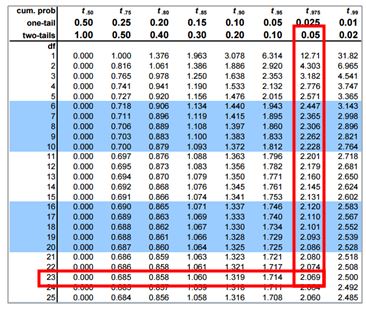
If the calculated t value is less than -2.069 or greater than 2.069, then reject the null hypothesis.
Test Statistic

I nterpret the results :
Compare t calc to t critical . In hypothesis testing, a critical value is a point on the test distribution compares to the test statistic to determine whether to reject the null hypothesis. Calculated t statistic value less than the critical value, hence failed to reject null hypothesis ( H 0 ). So, there is no significant difference between mean weights of apples in farm A and farm B.
Two Sample T 2 Tailed Equal Variance template file
Unlock additional members-only content, thank you for being a member, two sample t hypothesis test (unequal variance) videos.
Additional Two Sample T Hypothesis Tests Resources
- Good example of two sample T tests here.
- http://www.cliffsnotes.com/math/statistics/univariate-inferential-tests/two-sample-t-test-for-comparing-two-means (Two sample T test for comparing two means / DF for separate s: the smaller of n 1– 1 and n 2– 1 DF for pooled s: df = n 1+ n 2– 2)
I originally created SixSigmaStudyGuide.com to help me prepare for my own Black belt exams. Overtime I've grown the site to help tens of thousands of Six Sigma belt candidates prepare for their Green Belt & Black Belt exams. Go here to learn how to pass your Six Sigma exam the 1st time through!

Comments (7)
In the blood pressure question, can you please explain how you got 7.3 for s? No matter what I do, I am always getting to 7.08
Thanks for the head’s up, Jeremy. I see an opportunity for improvement on both of the examples listed. I’ll update asap.
I added additional detail in the calculation steps.
For these equations with so many variables I find it helpful to go slowly and write out the smaller operations of each part of the calculation.
Does this make sense?
the above states formula for Sample Variation as S2 = {( X Bar– x1)2 + (X Bar – x2)2 + … +(X Bar – xn)2} / n
however the IASSC Reference document is stating
S2 = {( X Bar– x1)2 + (X Bar – x2)2 + … +(X Bar – xn)2} / n-1
Could you please clarify
Thanks Maria
Thank you Maria,
When we divide by n in the sample variance S2, it is not an unbiased estimate of the population variance. Hence it is always recommended to use n-1 instead of n.
I have updated the formula
The formula for Two Sample T Hypothesis Test (Unequal Variance) formula that you have doesn’t match the formula shown on the IASSC formula sheet. Specifically A = sqrt(s1^2/n1), B = sqrt(s2^2/n2) and the way you’ve shown it you have A = s1^2/n1, B = s2^2/n2. Please update.
Hello Gariel Smith,
The formula and calculations are correct, we cross-checked with the Quality Council of Indiana Book as well as the below websites.
https://www.real-statistics.com/students-t-distribution/two-sample-t-test-uequal-variances/
https://www.theopeneducator.com/doe/hypothesis-Testing-Inferential-Statistics-Analysis-of-Variance-ANOVA/Two-Sample-T-Test-Unequal-Variance
Thanks Ramana
Leave a Reply Cancel reply
Your email address will not be published. Required fields are marked *
This site uses Akismet to reduce spam. Learn how your comment data is processed .
Insert/edit link
Enter the destination URL
Or link to existing content
COMMENTS
Fortunately, a two sample t-test allows us to answer this question. Two Sample t-test: Formula. A two-sample t-test always uses the following null hypothesis: H 0: μ 1 = μ 2 (the two population means are equal) The alternative hypothesis can be either two-tailed, left-tailed, or right-tailed:
Two-Sample T Test Hypotheses. Null hypothesis (H 0): Two population means are equal (µ 1 = µ 2). Alternative hypothesis (H A): Two population means are not equal (µ 1 ≠ µ 2). Again, when the p-value is less than or equal to your significance level, reject the null hypothesis. The difference between the two means is statistically significant.
How Two-Sample T-tests Calculate T-Values. Use the 2-sample t-test when you want to analyze the difference between the means of two independent samples. This test is also known as the independent samples t-test. Click the link to learn more about its hypotheses, assumptions, and interpretations. Like the other t-tests, this procedure reduces ...
The results for the two-sample t-test that assumes equal variances are the same as our calculations earlier. The test statistic is 2.79996. The software shows results for a two-sided test and for one-sided tests. The two-sided test is what we want (Prob > |t|). Our null hypothesis is that the mean body fat for men and women is equal.
Fortunately, a two sample t-test allows us to answer this question. Two Sample t-test: Formula. A two-sample t-test always uses the following null hypothesis: H 0: μ 1 = μ 2 (the two population means are equal) The alternative hypothesis can be either two-tailed, left-tailed, or right-tailed:
Revised on June 22, 2023. A t test is a statistical test that is used to compare the means of two groups. It is often used in hypothesis testing to determine whether a process or treatment actually has an effect on the population of interest, or whether two groups are different from one another. t test example.
Independent Samples T Tests Hypotheses. Independent samples t tests have the following hypotheses: Null hypothesis: The means for the two populations are equal. Alternative hypothesis: The means for the two populations are not equal.; If the p-value is less than your significance level (e.g., 0.05), you can reject the null hypothesis. The difference between the two means is statistically ...
And let's assume that we are working with a significance level of 0.05. So pause the video, and conduct the two sample T test here, to see whether there's evidence that the sizes of tomato plants differ between the fields. Alright, now let's work through this together. So like always, let's first construct our null hypothesis.
If that's below your significance level, then you would reject your null hypothesis and it would suggest the alternative that might be that, "Hey, maybe this mean "is greater than zero." On the other hand, a two-sample T test is where you're thinking about two different populations. For example, you could be thinking about a population of men ...
The independent t-test, also called the two sample t-test, independent-samples t-test or student's t-test, is an inferential statistical test that determines whether there is a statistically significant difference between the means in two unrelated groups. ... The null hypothesis for the independent t-test is that the population means from the ...
First of all, if you have two groups, one testing one placebo, then it's 2 samples. If it is the same group before and after, then paired t-test. I'm trying to run a dependent sample t-test/paired sample t test through using data from a Qualtrics survey measuring two groups of people (one with social anxiety and one without on the effects of ...
The 2-sample t-test takes your sample data from two groups and boils it down to the t-value. The process is very similar to the 1-sample t-test, and you can still use the analogy of the signal-to-noise ratio. Unlike the paired t-test, the 2-sample t-test requires independent groups for each sample. The formula is below, and then some discussion.
A one-sample t-test (to test the mean of a single group against a hypothesized mean); A two-sample t-test (to compare the means for two groups); or. A paired t-test (to check how the mean from the same group changes after some intervention). Decide on the alternative hypothesis: Two-tailed; Left-tailed; or. Right-tailed.
00:37:48 - Create a two sample t-test and confidence interval with pooled variances (Example #4) 00:51:23 - Construct a two-sample t-test (Example #5) 00:59:47 - Matched Pair one sample t-test (Example #6) 01:09:38 - Use a match paired hypothesis test and provide a confidence interval for difference of means (Example #7) Practice ...
15.1 Two Sample t test. We can also use the t test command to conduct a hypothesis test on data where we have samples from two populations. To introduce this lets consider an example from sports analytics. In particular, let us consider the NBA draft and the value of a lottery pick in the draft. Teams which do make the playoffs are entered into ...
The t-test for dependent samples is a statistical test for comparing the means from two dependent populations (or the difference between the means from two populations). The t-test is used when the differences are normally distributed. The samples also must be dependent. The formula for the t-test statistic is: t = D¯−μD (SD n√) t = D ...
If this is not the case, you should instead use the Welch's t-test calculator. To perform a two sample t-test, simply fill in the information below and then click the "Calculate" button. Enter raw data Enter summary data. Sample 1. 301, 298, 295, 297, 304, 305, 309, 298, 291, 299, 293, 304. Sample 2.
The T-test for Two Independent Samples More about the t-test for two means so you can better interpret the output presented above: A t-test for two means with unknown population variances and two independent samples is a hypothesis test that attempts to make a claim about the population means (\(\mu_1\) and \(\mu_2\)).
The two-sample t-test (Snedecor and Cochran, 1989) is used to determine if two population means are equal. A common application is to test if a new process or treatment is superior to a current process or treatment. ... In this case, we can state the null hypothesis in the form that the difference between the two populations means is equal to ...
Writing hypotheses to test the difference of means. An exercise scientist wanted to test the effectiveness of a new program designed to increase the flexibility of senior citizens. They recruited participants and rated their flexibility according to a standard scale before starting the program. The participants all went through the program and ...
by Zach Bobbitt August 3, 2022. A two sample t-test is used to test whether or not the means of two populations are equal. You can use the following basic syntax to perform a two sample t-test in R: t.test(group1, group2, var.equal=TRUE) Note: By specifying var.equal=TRUE, we tell R to assume that the variances are equal between the two samples.
A two sample t hypothesis tests also known as independent t-test is used to analyze the difference between two unknown population means. The Two-sample T-test is used when the two small samples (n< 30) are taken from two different populations and compared. The underlying chart makes use of the T distribution.
In statistics, Welch's t-test, or unequal variances t-test, is a two-sample location test which is used to test the (null) hypothesis that two populations have equal means. It is named for its creator, Bernard Lewis Welch, and is an adaptation of Student's t-test, and is more reliable when the two samples have unequal variances and possibly unequal sample sizes.