Partial molar volume
The aim is to determine the partial molar volume of water and sodium hydroxide within a binary mixture of the two components. The partial molar volume is then compared to the molar volume of the pure substances.

Molar volume
The molar volume of a pure substance V_\text{m}^\text{pure} is the ratio of volume V and the amount of substance n :
Generally, the molar volume V_\text{m} depends on pressure p and temperature T , since its volume V is pressure and temperature dependent. The molar volume of the ideal gas V_\text{m}^\text{ideal} is
since interaction between the gas molecules are neglected. The universal gas constant is R=8{.}314\,\text J\,/\,(\text{mol}\,\text K) . If the interactions between the particles of a pure substances cannot be neglected, the molar volume (equation ) deviates from the molar volume of an ideal gas (equation ). For liquids and solids the deviation is particularly pronounced.
Definition of the partial molar volume
Next we consider a homogeneous mixture of N different pure substances. The volume of the mixture depends on pressure and temperature. Furthermore, experimental data shows that the volume of the mixture additionally depends on the composition of the mixture.
The total differential of the volume of the mixture is:
Here, we denote the change in the mixture volume upon a change of the amount of substance of component i as partial molar volume V_{\text{m},i} .
The subscript p,T,n_{i\neq j} means that pressure, temperature and amount of substance of each other component is held constant. If the interaction between the particles of the mixture would be the same as within the pure substance, the partial molar volume would not depend on the composition and would thus equal the molar volume of the pure substance. In this case, the volume of the mixture would be the sum of the molar volume of the pure substances. If, however, there are different interactions between the particles of the mixture, the partial molar volumes V_{\text{m},i} are different from the molar volumes V_{\text{m},i}^{\text{pure}} of the pure substances:
The partial molar volumes are a function of pressure, temperature and composition of the mixture.
Binary mixtures
In this lab course a homogeneous mixture of water and sodium hydroxide is investigated. In this two-component mixture ( N=2 ) a change of the amount of substance of a single component ( \mathrm d n_1\neq 0 ) under constant pressure ( \mathrm d p=0 ) and constant temperature ( \mathrm d T=0 ) while keeping the amount of substance of the other component constant ( \mathrm d n_2=0 ) allows to determine the partial molar volume of the first component using equation .
For this it is necessary to measure the change in volume of the mixture V_\text{diff} upon addition of an amount of substance of the first component n_\text{1,diff} . Since the volume V of the binary mixture is
we can also determine the partial molar volume of the second component if we know each component's total amount of substance n_1 and n_2 :
By comparing the experimentally determined partial molar volumes from equations and with the molar volumes of the pure substances from equation we can determine whether, for example, the interaction between two water molecules is different compared to the interaction between water and sodium and hydroxide ions, respectively.
Experimental setup
Volume measurement apparatus.
The apparatus for mixing the two components and measuring the volume of the mixture is a vessel with a burette. A tap on the bottom of the vessel allows to fill the vessel with water from a reservoir. Using a funnel, the solid sodium hydroxide can be added to the water. The volume of the mixture is determined using the burette. The vessel is surrounded by a tempering jacket and additionally a heat exchange spiral is inside the vessel. This allows to keep the mixture at a constant Celsius temperature of 25 ℃ using a thermostat. The temperature can be checked using a thermometer, which is placed in a small glass inlet filled with water (such that the probe is not in contact with the sodium hydroxide solution). Below the vessel, a magnetic stirrer allows to speed up the dissolution of sodium hydroxide.
Degassing apparatus
At large concentration of sodium hydroxide the solubility of air in the mixture is less than in pure water. Using non-degassed (i.e. normal) water gas bubbles would form in the course of the experiment that influence the volume measurement. For this, deionized water is degassed with a diaphragm pump under stirring.
Solid sodium hydroxide is hygroscopic and is therefore portioned in a screw cap bottle. Determine the mass of the filled bottle. After adding the solid to the mixture the actually used mass is determined by weighing the empty bottle again and taking the difference.
Instructions
Virtual lab course video tutorial, lab course instructions, preparation.
Turn on the thermostat and set the Celsius temperature to 25 ℃. Make sure the cooling circulation is active.
Fill the round-bottom flask up until the mark using a funnel with deionized water. Using the diaphragm pump a vacuum is created to degas the water under stirring.
After the water has been degassed for ten to fifteen minutes the tap on the round-bottom flask is opened and the three-way cock is adjusted such that the water flows into the vessel. The burette should show a volume between 5 mL and 10 mL.
Turn on the magnetic stirrer and wait until the temperature of the mixture is constant.
Write down the environmental pressure, the Celsius temperature of the mixture and the volume of the burette.
Measuring the volume as function of added sodium hydroxide mass
Weigh a portion of approximately 10 g to 15 g of sodium hydroxide in the screw-top bottle. Work quickly, as sodium hydroxide is hygroscopic. Weigh the filled bottle, transfer the sodium hydroxide slowly and carefully via the burette into the vessel and weigh the empty bottle. The mass of the added sodium hydroxide is later determined by taking the mass difference.
Wait until the mixture is homogeneous and the temperature is constant. Note the Celsius temperature, the pressure and the burette volume. Make sure that the thermometer is immersed in the contact liquid (water).
If, after some time, there are still some pieces of sodium hydroxide left (not dissolved), note down the number of sodium hydroxide pieces and determine later the mass of a single sodium hydroxide piece to consider the number of undissolved pieces later in the analysis.
Repeat the above steps for a total of 8 additions of sodium hydroxide.
Turn off the thermostat and remove the mixture from the vessel.
Clean the vessel multiple times with deionized water. Take care that no sodium hydroxide pieces remain at the scale.
Clean up all equipment that has been in contact with sodium hydroxide.
Molar volume of the pure substances
Use equation and the following values for the molar mass M and density \rho to compute the molar volume of solid sodium hydroxide (index 1 ) and water (index 2 ) at \vartheta=25°\text C and p=101325\,\text{Pa} . Compare the computed molar volumes with the molar volume of the ideal gas (equation ).
Assume that the given values for the molar mass and the density are with error/uncertainty.
Calculation of the mixture volume
Determine the volume of the mixture by adding the measured burette volume to the volume of the vessel. At a burette volume of V_{\text{burette}} = 0\,\text{mL} the vessel volume is V=V_\text{vessel} = (994\pm0{.}05)\,\text{mL} . Compute the total amount of substance of sodium hydroxide n_1 after each addition of sodium hydroxide. Plot the mixture volume V (ordinate) against the amount of substance of sodium hydroxide n_1 (abscissa) and discuss the data. Compare with the volume of solid sodium hydroxide added to the mixture.
Determination of the partial molar volume
Determine the partial molar volume of sodium hydroxide V_{\text{m},1} using equation and the partial molar volume of water V_{\text{m},2} with equation . Calculate from the initial amount of substance of water n_2 and the respective amount of substance of sodium hydroxide n_1 in the mixture the mole fraction of sodium hydroxide x_1 . Plot the calculated partial molar volume (ordinate) against the mole fraction of sodium hydroxide (abscissa) in a single diagram. Discuss your data and compare with the molar volumes of the pure substances.
Vorbereitung auf das Kolloquium
Das Kolloquium beinhaltet zwei Themen. Bei beiden Themen wird vorausgesetzt, dass von den besprochenen Größen die physikalische Bedeutung, die Einheit und die Berechnung des zugehörigen Fehlers bekannt sind.
Erstes Thema: Erläutern Sie Versuchsziele, Versuchsdurchführung, verwendete Apparaturen und gemessene Größen.
Zweites Thema:
Wie bestimmen Sie experimentell das Gesamtvolumen der Mischung?
Wie wird das partielle Molvolumen von Natriumhydroxid und das partielle Molvolumen von Wasser berechnet?
Wie berechnet man das Molvolumen des idealen Gases?
Bibliography

An official website of the United States government
The .gov means it’s official. Federal government websites often end in .gov or .mil. Before sharing sensitive information, make sure you’re on a federal government site.
The site is secure. The https:// ensures that you are connecting to the official website and that any information you provide is encrypted and transmitted securely.
- Publications
- Account settings
Preview improvements coming to the PMC website in October 2024. Learn More or Try it out now .
- Advanced Search
- Journal List
- HHS Author Manuscripts
Determination of partial molar volumes from free energy perturbation theory †
Associated data.
Partial molar volume is an important thermodynamic property that gives insights into molecular size and intermolecular interactions in solution. Theoretical frameworks for determining the partial molar volume ( V °) of a solvated molecule generally apply Scaled Particle Theory or Kirkwood–Buff theory. With the current abilities to perform long molecular dynamics and Monte Carlo simulations, more direct methods are gaining popularity, such as computing V ° directly as the difference in computed volume from two simulations, one with a solute present and another without. Thermodynamically, V ° can also be determined as the pressure derivative of the free energy of solvation in the limit of infinite dilution. Both approaches are considered herein with the use of free energy perturbation (FEP) calculations to compute the necessary free energies of solvation at elevated pressures. Absolute and relative partial molar volumes are computed for benzene and benzene derivatives using the OPLS-AA force field. The mean unsigned error for all molecules is 2.8 cm 3 mol −1 . The present methodology should find use in many contexts such as the development and testing of force fields for use in computer simulations of organic and biomolecular systems, as a complement to related experimental studies, and to develop a deeper understanding of solute–solvent interactions.
Introduction
The partial molar volume of a substance, V i , in a solution depends on the temperature, pressure, and concentrations of all components. A particularly fundamental quantity is the partial molar volume of a substance in a pure solvent in the limit of infinite dilution, V °, which reflects the change in volume upon addition of a single solute molecule. Similarly, the free energy of solvation of the substance (Δ G solv ) corresponds to the change in free energy associated with its transfer from the gas phase into the solvent at infinite dilution. The two quantities are interrelated through the fundamental relationship, d G = V d P − S d T , such that at constant temperature, the pressure derivative of the free energy of solvation is equal to V ° ( eqn (1) ). 1 , 2 From a computational standpoint, one can then envision computation of V° via either
a direct calculation of the change in volume of a pure liquid upon adding the solute or by computing the free energy of solvation as a function of pressure. Such direct calculations were first performed when it became possible to carry out Monte Carlo statistical mechanics simulations in the NPT ensemble, e.g. , for methane in water and sodium and methoxide ions in methanol. 3 However, given the computer resources ca . 1980, the computed V ° values could not be adequately converged.
The situation has evolved, and today precise results can be obtained for both Δ G solv and V °. In particular, free energies of hydration have become increasingly used to evaluate the performance of molecular mechanic force fields, such as OPLS, AMBER, CHARMM, and AMEOBA. 4 – 14 Systematic studies of small molecule solvation are viewed as important tests for force-field parameters prior to their utilization in simulations of biological systems. However, computations of partial molar volumes and pressure and temperature effects on solution properties have not been regularly incorporated into force-field parameterization; rather they are sometimes investigated after the parameterization is complete. 15 – 20 This report focuses on the calculation of partial molar volumes, V °, by both the direct and derivative ( eqn (1) ) methods to establish optimal protocols and test some results for the OPLS-AA force field. 4 , 5
For additional background, it should be noted that theoretical frameworks that have been used to compute partial molar volumes of small molecules include Scaled Particle Theory (SPT), 21 Kirkwood–Buff theory (KBT), 22 and more direct techniques. 16 , 23 – 29 Each method has its advantages. 30 SPT yields an expression for the work of cavitation in hard sphere and real fluids, 31 and KBT can probe the local environment around a solute, giving insight into preferential solvation and solute–solvent interactions. 32 However, with the advancement of computational capabilities, more straightforward ways of estimating partial molar volumes are becoming popular. Floris in 2004 and Moghaddam and Chan in 2007 reinvestigated the direct method (DM) and showed that it could be used to obtain reliable results for hard-sphere cavities in water. 24 , 25 The direct method computes V ° as the difference between the total volume of N solvent plus one solute (A) molecules and the total volume of N solvent molecules alone. This can be done in two approaches. First, the position of the solute can be fixed (N, A) and the solute’s V ° can be determined from eqn (2) . The brackets 〈 V 〉 indicate total ensemble averages of volume; κ T represents the computed isothermal compressibility of the pure liquid; and, the last term in eqn (2) accounts for the contribution of translational motion of the solute, which amounts to 1.1 cm 3 mol −1 in water at 25 °C. 32 , 33 Alternatively, the solute can be allowed to freely translate and rotate through the solvent (N + A) and the solute’s V ° can be determined from eqn (3) . Since 2007, Weinberg and coworkers have similarly applied this methodology using molecular dynamics to analyze partial molar volumes of hydrocarbon solutes in a variety of solvents and volumes of activation for three reactions. 17 , 18 Additionaly, Ashbaugh and co-workers recently used the direct method in conjunction with other techniques to compute V ° values for amino acid side chains and volumes of micellization. 16 Others have employed this method to study thermodynamic properties of small proteins. 26 , 29
Alternatively, V ° can be determined by computing free energies of solvation at several pressures and fitting the data to a line ( eqn (1) ). In this report, this approach is referred to as the slope method, since V ° is given by the slope of the linear fit. Although most experimental partial molar volumes are determined via densitometric analyses, 34 – 37 the slope method has been applied experimentally to study very insoluble molecules in water. 38 Computationally, this approach has been less well explored than the direct methods. Moghaddam and Chan termed it the indirect method and used particle insertion to calculate methane’s free energy of hydration as a function of pressure, and thus methane’s V° via the slope of the linear fit. 24 Mohori and co-workers applied particle insertion methods and a thermodynamic perturbation theory with a hard-sphere reference to examine several thermodynamic properties of a 3D-Mercedes-Benz water model, including pressure and temperature derivative properties. They observed an “almost linear” relationship between transfer free energies and pressure. 15 Additionally, Dahlgren and co-workers have investigated several derivative properties of Na + and Cl − solvation free energies via thermodynamic integration. 39 However, in the present case free energy perturbation theory (FEP) based upon the Zwanzig equation 40 is applied to compute the requisite free energies of solvation.
With FEP theory, the free energy difference between an initial and final state of a system is computed as an ensemble average of the potential energy difference between those states, sampled at the initial state ( eqn (4) ). In Monte Carlo (MC) or molecular dynamics (MD) statistical mechanic simulations, FEP theory can be applied to study chemical equilibria via a thermodynamic cycle ( Scheme 1 ). 11 , 40 – 44 In this way, FEP theory has been used successfully to compute relative or absolute free energies of solvation for many small organic molecules. 9 – 11 , 43 In conjunction with the thermodynamic cycle in Scheme 1 , a relative free energy of solvation (ΔΔ G solv ) between two molecules can be calculated by transforming molecule (A) into a different molecule (B) in the gas phase and solution ( eqn (5) ). 11 , 40 – 44 An absolute free energy of solvation is computed in a similar manner, except that the final state of the perturbation (B) is a “null” or non-existent molecule; in this case Δ G B = 0 and eqn (6) applies. These calculations are often referred to as molecular annihilations and effectively make a molecule “disappear” from the gas phase and solution in separate calculations. 9 Computationally, the gas phase is treated as an ideal gas at a temperature of 25 °C and a pressure of 1 atm using a single molecule in isolation.

The slope method can be applied with FEP theory to determine a molecule’s partial molar volume by combining eqn (1) and (6) with Δ G solv = Δ G A and noting that ( d Δ G gas d P ) T = 0 in the ideal gas phase, thus yielding eqn (7) . Operationally, one needs to perform the annihilations of the solute in the solvent as a function of external pressure in the NPT ensemble and fit the free energy results to a line. In a similar manner, differences in partial molar volumes (Δ V °) for two solutes A and B can be obtained from relative FEP calculations using eqn (1) and (5) .
In this report, the slope method is used to evaluate the precision of FEP theory for computing partial molar volumes in explicit-solvent condensed phase simulations. This work uses much of the same methodology that has been reported previously for computing free energies of hydration at 25 °C, 9 – 11 , 43 except that simulations are also run at several pressures above 1 atm. Partial molar volumes computed via FEP theory are compared with results from the direct methods.
Computational details
All Monte Carlo simulations and free energy perturbation calculations were carried out with the BOSS program using the isothermal–isobaric ensemble at 25 °C. 45 Water was represented using the TIP4P water model. 46 All other solvents and solute molecules were represented with the OPLS-AA force field. 4 , 5 , 47 , 48 Prior to computing Δ G solv values at elevated pressures, pure liquid simulations of water, carbon tetrachloride, and benzene solvents were conducted to equilibrate all solvent boxes at elevated pressures. Direct method and FEP calculations ensued.
Pure liquid simulations
Metropolis MC simulations 49 were performed at increasing pressures for pure water, carbon tetrachloride (CCl 4 ), and benzene. Pressures in water ranged from 1 to 8000 atm in increments of 1000 atm. Pressures in carbon tetrachloride and benzene were performed up to 1000 atm and 650 atm, respectively, in increments of 150–250 atm. Reduced pressures for non-aqueous solvents were used to conform to experimental freezing pressures. At 25 °C, water freezes at ca . 9500 atm; 50 – 52 CCl 4 freezes at 1314 atm; 53 and benzene freezes at 703–725 atm. 53 , 54 These limits for CCl 4 and benzene have been generally well observed in several thermophysical studies. 55 – 58 Computed densities at elevated pressures show excellent agreement when compared to experiment ( Tables S1–S3 and Fig. S1–S3, ESI † ). 50 , 55 , 56 , 59 , 60 With the TIP4P model, the maximum percent error is 1.6%; the density of water is slightly overestimated at all pressures. For carbon tetrachloride and benzene the computed densities fall below the experimental values at all pressures and show maximum percent errors of 4.3% and 1.8%, respectively. This data suggests that TIP4P and OPLS-AA models are reasonably well-suited for volumetric studies at elevated pressures.
Simulations were carried out using cubic cells of 267 or 512 solvent molecules with periodic boundary conditions; the larger box was used for TIP4P water. Solvent molecules freely translated and rotated, but their intramolecular degrees of freedom were not sampled. Attempted changes in the volumes of the system were automatically adjusted by the program to achieve acceptance rates of ca . 40%, and the ranges for translations and rotations were set to yield acceptance rates of 40–50%. Solvent–solvent cutoff distances of 10 Å were used for water and CCl 4 , and a cutoff distance of 12 Å was used for benzene. Nonbonded cutoff distances are based on center-of-mass separations or the O–O distance for water and include quadratic smoothing to zero over the last 0.5 Å. 4 , 9 For non-aqueous solvents, the BOSS program automatically includes an energy correction to account for long-range Lennard-Jones interactions neglected beyond cutoff distances. 45 To ensure proper convergence at higher pressures, all simulations were equilibrated for 100 million (M) configurations, after which the averaging was continued for another 120 million configurations (100 M/120 M). 61 Simulations of water and CCl 4 began from stored solvent boxes in BOSS; neat benzene was generated as a custom solvent. Equilibrated solvent boxes for each pressure were subsequently used in the FEP calculations.
Direct method
Due to the ease and general success of estimating partial molar volumes directly from total simulation volumes, 16 – 19 , 24 , 25 , 33 the direct method was used to compute the partial molar volume of benzene in water, carbon tetrachloride, and benzene. To test convergence, calculations were performed using 20 M/20 M, 50 M/50 M, 100 M/100 M, 250 M/250 M, 500 M/500 M, 800 M/800 M and 1000 M/1000 M configurations. Cubic cells of 500 water, 264 CCl 4 , and 266 benzene solvent molecules were used with periodic boundary conditions. For simulations involving a benzene solute, solute–solvent cutoff distances were set to 10 Å and quadratic smoothing was performed over the last 0.5 Å of the cutoff. Solute moves were attempted every 100 steps and solute translations and rotation ranges were set to ±0.06 Å and ±6.0°. Internal degrees of freedom of the solute were fully sampled. All other simulation conditions are identical to those used in the pure liquid simulations, except that these simulations were performed only at 1 atm. For each solvent, three calculations were performed: solvent with no solute ( V N ), solvent with a fixed-position solute ( V N,A ), and solvent with an unrestrained solute ( V N+A ), corresponding to eqn (2) and (3) . 24 Statistical uncertainties (±1 σ ) were calculated from the batch means procedure using batch sizes of 1–5 M configurations. 11 , 62
Monte Carlo/free energy perturbations
Relative and absolute free energies of hydration were computed with the BOSS program using MC/FEP calculations, as described previously. 9 – 11 , 42 , 43 Alchemical transformations were performed in gas and solution according to the thermodynamic cycle in Scheme 1 to compute relative or absolute free energies. First, absolute Δ G solv values for water, CCl 4 , and benzene were computed in their respective neat liquid via complete annihilation. Δ G solv values for benzene in water and carbon tetrachloride were also determined in the same manner. Second, relative values, ΔΔ G solv , were computed by alchemically transforming benzene derivatives into benzene in the gas phase and in water. The pressure dependence of Δ G solv or ΔΔ G solv was then analyzed to derive partial molar volumes of all solutes.
Absolute Δ G solv values were determined in the three solvents at all pressures as described in the above pure liquid section. Benzene was selected for study in all three solvents due to its hydrophobic nature, the availability of experimental data, 34 , 35 , 38 , 63 – 65 and its inclusion in previous studies. 11 , 17 , 18 , 38 , 48 , 66 – 68 Water and CCl 4 were also examined in their pure liquids to help validate the methodology. To annihilate a molecule, all force field intermolecular interactions for the solute must be scaled to zero. This is best accomplished in two separate steps. First, all partial atomic charges are scaled to zero to remove the electrostatic contribution. Second, in a separate calculation, all Lennard-Jones parameters are scaled to zero while simultaneously shrinking the molecule. In the second step, solute shrinking is accomplished over the course of the simulation by perturbing all atom types to idealized sp 2 or sp 3 dummy atoms with equilibrium bond lengths of 0.3 Å. Each step of the annihilation was performed using twenty-one λ windows of simple overlap sampling (21-SOS) 11 , 69 with 8 M/8 M configurations in the gas phase and 30 M/75 M configurations in solution. 9 To avoid endpoint problems in the final window, SOS sampling was performed up to λ = 0.99 and double-wide sample (DWS) was used to complete the transformation ( λ = 0.99 → 1.00). Statistical uncertainties (±1 σ ) were calculated using batch sizes of 1 M configurations. 11 , 62 For individual computed Δ G solv values, the maximum uncertainty is below 0.25 kcal mol −1 , which is comparable to typical experimental uncertainties of 0.3 kcal mol −1 near ambient conditions. 70 , 71
For each Δ G solv , a single solute molecule was placed in a box of 500 water, 264 CCl 4 , or 266 benzene solvent molecules to enable consistent comparison with results obtained from the direct method. Equilibrated solvent boxes from the above pure liquid simulations provided the initial solvent coordinates. All solvent and solute simulation conditions mirror those described above in the Pure liquid and Direct method sections. Again, all internal degrees of freedom of the solute were fully sampled, and all solvent molecules were internally rigid. Once absolute free energies of solvation were obtained for all solutes at all pressures, V ° was determined from the slope of the best fit line ( eqn (1) ). Units of kcal mol −1 atm were converted to cm 3 mol −1 , the normal experimental units.
Relative ΔΔ G solv for several benzene derivatives were computed in water up to 4000 atm in increments of 500 atm. These calculations used 21-SOS sampling with no end-point modifications and 8 M/8 M configurations in the gas phase and 15 M/30 M configurations in solution. Decoupling of the electrostatic and Lennard-Jones perturbations is not needed. All other simulation details were identical as described above. Linear fits of the data were used to determine Δ V ° for the perturbations.
Direct method comparison
In this work, benzene was modeled in three solvents and the total average volumes from the simulations were used in eqn (2) and (3) . Because the total volume fluctuates during the simulations and the difference between two large numbers is being taken, high standard uncertainties are expected, if enough statistical sampling is not performed. 3 The convergence of the results was investigated by increasing the lengths of the MC runs as summarized in Table 1 .
Computed partial molar volumes (cm 3 mol −1 ) of benzene from the direct methods at 25 °C and 1 atm
| Number of configurations | Average total volume | 10 | ° ( ) | ° ( ) | ||
|---|---|---|---|---|---|---|
| Water | ||||||
| 20 M/20 M | 14917.3 | 15040.3 | 15006.0 | 38.7 | 74.1 ± 21.0 | 53.4 ± 19.2 |
| 50 M/50 M | 14910.9 | 15019.1 | 15077.2 | 54.8 | 65.2 ± 16.3 | 100.1 ± 17.3 |
| 100 M/100 M | 14895.9 | 15053.7 | 15053.1 | 53.6 | 95.0 ± 14.3 | 94.7 ± 14.5 |
| 250 M/250 M | 14937.2 | 15057.1 | 15062.7 | 48.9 | 72.2 ± 8.5 | 75.6 ± 8.9 |
| 500 M/500 M | 14925.9 | 15064.0 | 15038.5 | 46.9 | 83.2 ± 6.1 | 67.8 ± 6.1 |
| 800 M/800 M | 14918.6 | 15061.8 | 15056.6 | 51.5 | 86.3 ± 5.8 | 83.1 ± 5.7 |
| 1000 M/1000 M | 14918.4 | 15064.0 | 15053.2 | 50.7 | 87.7 ± 5.2 | 81.2 ± 5.1 |
| Expt. | 45.8 | 83.1 | 83.1 | |||
| Carbon tetrachloride | ||||||
| 20 M/20 M | 43323.0 | 43419.7 | 43411.3 | 108.6 | 58.2 ± 36.7 | 53.2 ± 28.8 |
| 50 M/50 M | 43220.5 | 43424.3 | 43412.3 | 116.2 | 122.7 ± 21.6 | 115.5 ± 21.8 |
| 100 M/100 M | 43277.5 | 43396.2 | 43391.4 | 116.8 | 71.5 ± 17.1 | 68.6 ± 17.0 |
| 250 M/250 M | 43257.1 | 43386.5 | 43408.3 | 120.6 | 77.9 ± 12.0 | 91.1 ± 11.8 |
| 500 M/500 M | 43259.8 | 43409.2 | 43411.0 | 118.7 | 90.0 ± 7.6 | 91.0 ± 7.5 |
| 800 M/800 M | 43273.6 | 43422.1 | 43400.0 | 121.5 | 89.4 ± 6.4 | 76.1 ± 6.4 |
| 1000 M/1000 M | 43260.3 | 43403.1 | 43410.2 | 119.7 | 86.0 ± 6.2 | 90.2 ± 5.9 |
| Expt. | 108.9 | 90.5 | 90.5 | |||
| Benzene | ||||||
| 20 M/20 M | 39641.5 | 39766.3 | 39838.3 | 107.3 | 75.1 ± 43.1 | 118.5 ± 40.1 |
| 50 M/50 M | 39789.2 | 39888.7 | 39875.4 | 101.2 | 59.9 ± 23.9 | 51.9 ± 24.1 |
| 100 M/100 M | 39720.1 | 39833.7 | 39876.1 | 109.4 | 68.4 ± 21.3 | 93.9 ± 20.3 |
| 250 M/250 M | 39704.8 | 39854.1 | 39840.0 | 98.4 | 89.9 ± 12.2 | 81.4 ± 12.0 |
| 500 M/500 M | 39727.1 | 39818.5 | 39843.9 | 103.9 | 55.1 ± 9.4 | 70.4 ± 9.8 |
| 800 M/800 M | 39700.5 | 39858.6 | 39859.3 | 102.7 | 95.2 ± 7.8 | 95.6 ± 7.8 |
| 1000 M/1000 M | 39700.1 | 39851.3 | 39844.3 | 103.6 | 91.0 ± 7.1 | 86.9 ± 7.1 |
| Expt. | 98.2 | 89.5 | 89.5 | |||
To obtain converged properties such as the density and heat of vaporization of a pure liquid via MC methods, 20 M/20 M configurations are generally considered sufficient for simulations run at 1 atm. 4 , 72 However, the uncertainties for V ° are seen to be 20–40 cm 3 mol −1 with this sampling. Increasing the sampling up to 1 billion configurations (1000 M) appears to be necessary to reduce the uncertainties to a few cm 3 mol −1 . Even between 500 M and 800 M configurations, the results from eqn (3) change by 15.3 cm 3 mol −1 in water, 14.9 cm 3 mol −1 in CCl 4 , and 25.2 cm 3 mol −1 in benzene. There is no striking difference in convergence using eqn (2) or (3) , though in general allowing the solute to translate and rotate in MC simulations is advantageous for convergence of solute–solvent properties such as radial distribution functions. Altogether, the results suggest that at least 1000 M configurations should be used with the present system sizes for determining partial molar volumes via the direct methods. Statistical uncertainties of ±6 cm 3 mol −1 are suggested by the results in Table 1 at this length. The results for V ° also have good accuracy with average discrepancies of 3 cm 3 mol −1 with the experimental data, which is consistent with the small errors ( ca . 2%) that are normally obtained for pure liquids with the OPLS-AA force field. 4 Longer simulations were not pursued here. In research by others, up to 10 billion MC configurations have been used for averaging, 3 , 24 while MD simulations of 40–500 ns have been used to compute V ° values. 16 – 18 In both cases, the statistical uncertainties remain near 3 cm 3 mol −1 . For comparing direct method results with those from the MC/FEP calculations, the V ° values computed with 1000 M configurations will be used.
Absolute free energies of solvation
Absolute free energies of solvation were determined for water in water, CCl 4 in CCl 4 , and benzene in the three solvents as a function of pressure ( Table 2 ). The computed free energies of hydration at 1 atm show errors of 0.2–1.6 kcal mol −1 . These errors are consistent with previous results with OPLS force fields, although the error for benzene in water is somewhat higher than previously reported. 10 , 14 For the present simulations, long-range Lennard-Jones corrections for benzene in water amount to 0.59 kcal mol −1.41,73 This correction would lower benzene’s free energy of hydration to 0.16 kcal mol −1 , which is in statistical agreement with previous calculations. Unfortunately, few experimental free energies of solvation are available at high pressures. The results for water in water and benzene in water are also plotted in Fig. 1 . There is no clear curvature, which implies that V ° is relatively constant over this pressure range ( eqn (1) ). Assuming this constancy, estimates of experimental free energies of solvation at elevated pressure can then be made from the observed V ° and Δ G solv at 1 atm. Table S4 ( ESI † ) lists such estimated results for Δ G solv for all present solutes and solvents at high pressure. The unsigned errors between the computed and the estimated experimental Δ G solv values are well maintained as pressure increases.

Computed free energies of solvation (kcal mol −1 ) for water in water (red) and benzene in water (blue) vs . external pressure (atm); dashed lines represent best fit lines; R 2 = 0.997 (water) and 0.998 (benzene).
Computed free energies of solvation (kcal mol −1 ) in three solvents with increasing external pressure (atm) at 25 °C a
| Water | Carbon tetrachloride | Benzene | |||||
|---|---|---|---|---|---|---|---|
| Pressure | Δ (H O) | Δ (C H ) | Pressure | Δ (CCl ) | Δ (C H ) | Pressure | Δ (C H ) |
| 1 | −6.13 | 0.75 | 1 | −3.58 | −3.40 | 1 | −3.59 |
| 1000 | −5.77 | 2.89 | 250 | −3.01 | −2.78 | 50 | −3.30 |
| 2000 | −5.32 | 4.73 | 500 | −2.46 | −2.30 | 200 | −3.08 |
| 3000 | −5.03 | 6.71 | 750 | −1.83 | −1.80 | 350 | −2.66 |
| 4000 | −4.52 | 8.40 | 1000 | −1.14 | −1.29 | 500 | −2.36 |
| 5000 | −4.33 | 10.49 | 650 | −2.26 | |||
| 6000 | −3.87 | 12.17 | |||||
| 7000 | −3.57 | 13.47 | |||||
| 8000 | −3.15 | 16.02 | |||||
Partial molar volumes
The relationship between free energy and pressure is expected to deviate from linearity at high pressures, especially in organic solvents which are more compressible than water. However, the effect is not obvious in the present results ( Fig. 1 ), and the data can be modelled well with linear equations ( R 2 > 4 0.90). Quadratic fits of the data ( Table 2 ), which account for solvent compressibility, were also performed. However, high error estimates were observed for the quadratic coefficients. The magnitude of the predicted uncertainty was generally greater than or equal to the intrinsic value of the coefficient, indicating that this parameter is not well described by the data. 74 Similar difficulties have been described previously. 39 Thus linear fits were chosen for data analysis; the slope yields V °. This analysis is similar to that performed for reactions under high pressure, where the volume change corresponds to the volume of activation. 2 , 75 , 76 In computing volumes of activation, Eckbert suggested using data below a limit of 10% compression of the solvent. 75 For TIP4P water, 10% compression is reached around 4000 atm, and thus linear fits to determine V ° in water were restricted to data in the range of 1–4000 atm. The pressure ranges were smaller for carbon tetrachloride and benzene with compressions less than 10%, so all computed data were used.
Because the molecular annihilations decouple electrostatic and van der Waals interactions of the solute in two separate calculations, the effects of pressure on both components were obtained. Using benzene in water as an example, Fig. S4 ( ESI † ) shows that the linear increase of Δ G solv is dominated by the van der Waals (Lennard-Jones) component, while the free energy change for neutralizing all atoms of the solute is essentially constant at −1.9 kcal mol −1 ( Table S5, ESI † ). Thus, the computed V ° values are highly dependent on the Lennard-Jones parameters used to model a solute and the linear increase of Δ G solv with pressure is a volume effect. It becomes increasingly difficult to create a cavity for the solute with increasing pressure.
To investigate the precision of obtaining V ° from the slope method, single molecules were first annihilated in their pure liquids. V ° values were determined from the slopes of the data in Table 2 and compared to the molar volume of a single solvent molecule from the respective pure liquid simulations ( Table 3 ). The molar volume of a single solvent molecule from a pure liquid simulation is determined by dividing the average total volume of the pure solvent box by the number of solvent molecules in the box ( V total /N). V ° should equal V total /N within the statistical uncertainty. For both TIP4P water and CCl 4 , V ° is ca . 1.5 cm 3 mol −1 less than V total /N. The uncertainty for V ° can be approximated from the standard error of the estimate that is obtained from the linear fit. 74 For V ° determined in water or carbon tetrachloride solvents, the estimated uncertainty is ca . 1.8 cm 3 mol −1 ; for benzene in benzene the uncertainty increases to 8.0 cm 3 mol −1 . Thus, the accord between the computed V ° and V total /N values is reasonable, and the statistical uncertainties are similar to those from the longest direct method results in Table 1 . It is also pleasing that the computed V ° values for benzene in water (79.0), benzene (84.8), and carbon tetrachloride (86.1) are in the same order as observed experimentally; the computed values are uniformly 4–5 cm 3 mol −1 too low. The V ° values for carbon tetrachloride and benzene in carbon tetrachloride are also in the right order. In view of the statistical uncertainties, this may all be serendipitous, though it does encourage further study and application of the slope method. Similarly, if one averages the results from the 1000 M/1000 M direct calculations, the computed V ° values for benzene in water, benzene, and carbon tetrachloride are 84.5, 89.0, and 88.1 cm 3 mol −1 , which has the order of the last two values switched. In both cases, an important qualitative prediction is correct, i.e. , that the partial molar volume of benzene in water is smaller than in the other solvents. This can be interpreted as reflecting a hydrophobic effect that aims to reduce the surface area of water molecules in contact with benzene and/or a solvent size effect whereby smaller molecules can form more compact arrangements about an object than larger molecules, like peas vs . oranges.
Calculated partial molar volumes (cm 3 mol −1 ) of water, CCl 4 , and benzene in solution from the slope method ( eqn (1) ) and pure liquid simulations at 25 °C
| Solute | Solvent | ° | /N | Expt. ° |
|---|---|---|---|---|
| Water | Water | 16.3 | 18.0 | 18.1 |
| CCl | CCl | 100.1 | 101.4 | 97.0 |
| Benzene | Benzene | 84.8 | 91.0 | 89.5 |
| Benzene | Water | 79.0 | – | 83.1 |
| Benzene | CCl | 86.1 | – | 90.5 |
Relative partial molar volumes
In addition to computing partial molar volumes by annihilating entire molecules in solution, relative FEP calculations provide a means to estimate differences in partial molar volumes (Δ V °). By computing ΔΔ G solv at increasing pressures, Δ V ° can be estimated from the slope of the fit. This is illustrated here for derivatives of benzene in water. As shown in Table 4 , computed relative free energies of hydration for benzene derivatives at 1 atm with the OPLS-AA force field are in excellent agreement with experimental results. 11 , 70 The mean unsigned error is 0.44 kcal mol −1 , and the largest error (1.08 kcal mol −1 ) is for nitrobenzene relative to benzene. Computed ΔΔ G hyd values were then obtained at increasing pressures up to 4000 atm, as reported in Table S6 ( ESI † ).
Computed relative partial molar volumes (cm 3 mol −1 ) in water from the slope method a
| Ph–X→Ph–Y | ΔΔ (kcal mol ) | Δ ° (cm mol ) | |||
|---|---|---|---|---|---|
| Computed | Expt. | Computed | Expt. | ||
| CH | H | 0.31 ± 0.03 | 0.03 | −15.2 | −13.9 |
| F | H | −0.27 ± 0.02 | −0.06 | −2.9 | −8.4 |
| Cl | H | −0.44 ± 0.03 | 0.26 | −11.7 | |
| OH | H | 5.14 ± 0.05 | 5.76 | −2.0 | −1.8 |
| NH | H | 4.40 ± 0.04 | 4.63 | +1.6 | −6.4 |
| OCH | H | 0.65 ± 0.06 | 1.60 | −22.0 | −22.5 |
| CHO | H | 3.12 ± 0.08 | 3.16 | −13.0 | −13.7 |
| COCH | H | 3.08 ± 0.10 | 3.72 | −26.0 | −29.9 |
| NO | H | 2.18 ± 0.07 | 3.26 | −11.9 | −13.0 |
| OCH | OH | −4.50 ± 0.07 | −4.16 | −21.3 | −20.7 |
| NHMe | NH | −0.90 ± 0.06 | −0.80 | −19.1 | −17.7 |
| NMe | NHMe | −0.91 ± 0.06 | −1.24 | −15.3 | −16.5 |
| COCH | CONH | −6.68 ± 0.06 | −6.43 | −16.9 | −10.6 |
| CONHMe | CONH | −2.99 ± 0.07 | −21.0 | −17.8 | |
| CONMe | CONHMe | −2.80 ± 0.07 | −21.0 | −17.0 | |
| Mean unsigned error | 0.44 | 2.7 | |||
The resultant computed Δ V ° values are also in good agreement with experiment ( Table 4 ). The mean unsigned error is 2.7 cm 3 mol −1 , and the statistical uncertainties are 1.0–2.0 cm 3 mol −1 . In all cases, the R 2 values for the linear fits are above 0.84, with half greater than 0.95. The linear fits for phenol and aniline have R 2 values less than 0.50 and are discussed below. Experimental Δ V ° values are derived from the V ° of benzene in water determined by Masterson 34 and the values for benzene derivatives from Shahidi. 65 Although Shahidi reports the V ° of benzene as 81.3 cm 3 mol −1 , 65 a variety of literature sources suggest it is closer to the value reported by Masterson; 35 , 38 , 66 , 77 thus 83.1 cm 3 mol −1 was used for the V ° of benzene in water.
The calculations in best agreement with experiment generally involve the appearance or disappearance of a methyl group. For example, Δ V ° results for perturbing toluene to benzene, anisole to phenol, N -methylaniline to aniline, and N , N -dimethylaniline to N -methylaniline all show errors of 1.4 cm 3 mol −1 or less. Errors are somewhat higher for the benzamide series. Perturbing N , N -dimethylbenzamide to N -methylbenzamide or N -methylbenzamide into benzamide gives errors of 3.0–4.0 cm 3 mol −1 . For both cases, there are no significant differences in the Lennard-Jones parameters between the initial and final molecules, aside from the CH 3 to H mutation, and the data are all well fit by linear models ( R 2 > 0.930). For all H to CH 3 conversions, the average Δ V ° for methylation is 17.7 cm 3 mol −1 , which is in excellent agreement with experiment, 17.3 cm 3 mol −1.65
Other computed results which show close accord with experiment include anisole to phenol and anisole to benzene with errors of ca . 0.5 cm 3 mol −1 , and benzaldehyde to benzene, where the error is 0.7 cm 3 mol −1 . For acetophenone to benzene and nitrobenzene to benzene, larger transformations that simultaneously mutate three non-hydrogen atoms, the errors are 3.9 and 1.1 cm 3 mol −1 , respectively. Altogether these results indicate that the MC/FEP calculations are robust for determining Δ V °, even when several non-hydrogen atom are mutated simultaneously.
A peculiarity of the current data is the results for phenol and aniline ( Table 4 ). Although the error for phenol to benzene is only 0.2 cm 3 mol −1 , the error for aniline to benzene is 8.0 cm 3 mol −1 . A significant amount of scatter is present in the data, as represented by low correlation coefficients for the linear fits of the pressure results ( R 2 < 0.50). Such transformations have a large impact on the solute–water interactions since a strongly hydrogen bonding group is being fully deleted. Convergence for the solvent structure and Δ V ° is expected to be more difficult in such cases. Thus, it is possible that the small error for phenol to benzene is coincidental. Notably, when an absolute V ° for phenol in water is determined via molecular annihilation, similar to benzene above, a V ° of 78.3 cm 3 mol −1 is obtained ( R 2 = 0.996). From phenol’s and benzene’s independently calculated V ° values, Δ V ° for phenol to benzene is then +0.7 cm 3 mol −1 , which gives an error of 2.5 cm 3 mol −1 . This is likely a better estimate of the error due to the improved linear fit of the absolute calculations. In order to obtain more precise results in cases where there is a large change in hydrogen bonding, it is advisable to perform longer runs or to perform the perturbations in smaller steps, e.g. , OH to F to H.
Conclusions
The results presented here show that estimates of a molecule’s partial molar volume may be readily obtained using MC simulations and either the direct methods ( eqn (2) and (3) ) or the slope method ( eqn (1) ) to a precision of a few cm 3 mol −1 . Direct method calculations are more straightforward and require only one simulation per solute once the volume of the solvent system has been determined. Calculations performed on an Intel Core2 3.3 GHz processor with the BOSS program required ca . 7.5 hours for 1000 M configurations of averaging. The additional 1000 M configurations of equilibration that was used is excessive; ca . 200 M would suffice. Thus, using 4 processors with independent runs, one could obtain results for 4000 M configurations of averaging in about 8 hours or 12 billion configurations in a day. It is of historical interest to note that for the earliest calculations of this type, only 0.7 M and 2 M configurations of averaging were executed for systems with 100 or 127 solvent molecules. 3
To determine V ° for a single solute with the slope method, the current protocol used at least twelve calculations: two gas phase calculations at 1 atm, and two condensed phase calculations for each of five pressure increments. On the same Intel processor, one FEP window for the liquid phase takes about 70 minutes; and, the full 21-SOS annihilation requires ca . 30.2 hours when all windows are run sequentially on one processor. Thus, on one processor the current slope calculations took about 12 days per molecule, i.e. , 30–40 times longer than the direct calculations for similar precision. This could be sped up by only using three pressures rather than five, and the FEP calculations are readily parallelizable by running different windows on different processors. However, the slope method is competitive for computation of differences in V ° values since the full annihilations are replaced by small perturbations. This was illustrated for the substituted benzenes where the unsigned errors compared to experimental data averaged only 2.7 cm 3 mol −1 . In view of the shorter runs and lack of electrostatic decoupling, the relative FEP calculations needed only about 35 minutes per FEP window or ca . 10 hours for a complete calculation. If three pressures were used, the total calculation time would be 30 hours, which is likely shorter than the direct calculations that would be required to yield a similar level of precision for the difference in V ° values for the two molecules. Operationally, it is easy to parallelize both types of calculations, so many molecules could be processed in one day with reasonable resources.
Concerning accuracy, the present results supported the quality of the TIP4P and OPLS-AA models for problems associated with liquid densities. For benzene in the three solvents, the average error in V ° from the direct calculations is 3.0% ( Table 1 ) and it is 5.0% for the slope calculations ( Table 3 ), which are similar to the statistical uncertainties in the results. Further calculations of partial molar volumes should find use in force field development and in developing an enhanced understanding of solute–solvent interactions.
Supplementary Material
Acknowledgments.
Gratitude is expressed to the National Institutes of Health (GM32136) for support of this work, and to Daniel J. Cole, John C. Faver, and Michael J. Robertson for helpful discussions.
† Electronic supplementary information (ESI) available: Supplementary tables and figures have been provided containing detailed thermodynamic results for liquid densities as a function of pressure and partial molar volumes (8 pages). See DOI: 10.1039/c4cp05304d
Academia.edu no longer supports Internet Explorer.
To browse Academia.edu and the wider internet faster and more securely, please take a few seconds to upgrade your browser .
Enter the email address you signed up with and we'll email you a reset link.
- We're Hiring!
- Help Center

Partial molal volume

CHEM 171.42 Physical Chemistry I, laboratory 1st sem, A.Y. 2020-2021 Ateneo de Manila University
Related Papers
Jonniel Vince Cruz
This experiment aimed to know the partial molar volume of sodium chloride (NaCl) and water in the solution at different molar concentrations. Using simple mixing rules for non-ideal solution is greatly erroneous, that is why partial molar volumes are determined. This method is used to predict what changes occur upon changing the composition of a solution.
Paul Asimow
Journal of Solution Chemistry
Charles Oakes
Journal of Chemical & Engineering Data
Frank Millero
Fluid Phase Equilibria
Luca Bernazzani
Chemical physics letters
Raji Heyrovska
Ramesh L . Gardas
AFIFAH FAUZI
afifah fauzi
Abdullah M. Asiri
Loading Preview
Sorry, preview is currently unavailable. You can download the paper by clicking the button above.
RELATED PAPERS
Giannis Papaefstathiou
Piotr Gauden
Journal of Chemical and Engineering Data - J CHEM ENG DATA
gianfrancesco berchiesi
Ivan Jimenez
The Journal of Chemical Thermodynamics
Sharad Sharma
Dr Zikhona Tywabi-Ngeva
Jaber Jahanbin
Ajaya Bhattarai
The Journal of Chemical Physics
Giuseppe Graziano
Thiviaraj Palani
Journal of Thermal Analysis and Calorimetry
Ezequiel Sarid Jiménez
Thermochimica Acta
Indra Bahadur
Luigi Bubacco
anam fatima
Pratyush kHANDELWAL
Ramsharan Singh
Jaquelin Hernandez
Quantitative Structure-Activity Relationships
harrie govers
RELATED TOPICS
- We're Hiring!
- Help Center
- Find new research papers in:
- Health Sciences
- Earth Sciences
- Cognitive Science
- Mathematics
- Computer Science
- Academia ©2024
Thank you for visiting nature.com. You are using a browser version with limited support for CSS. To obtain the best experience, we recommend you use a more up to date browser (or turn off compatibility mode in Internet Explorer). In the meantime, to ensure continued support, we are displaying the site without styles and JavaScript.
- View all journals
- Explore content
- About the journal
- Publish with us
- Sign up for alerts
- Published: 21 August 2024
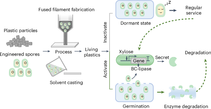
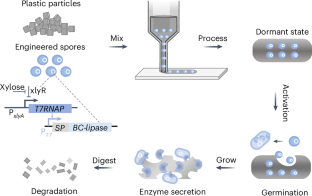
Degradable living plastics programmed by engineered spores
- Chenwang Tang 1 , 2 ,
- Lin Wang 1 na1 ,
- Jing Sun 2 , 3 na1 ,
- Guangda Chen 4 ,
- Junfeng Shen 1 ,
- Liang Wang 5 ,
- Ying Han 1 ,
- Jiren Luo 1 ,
- Zhiying Li 5 ,
- Pei Zhang 4 ,
- Simin Zeng 1 ,
- Dianpeng Qi 2 ,
- Jin Geng ORCID: orcid.org/0000-0003-2181-0718 5 ,
- Ji Liu ORCID: orcid.org/0000-0001-7171-405X 4 &
- Zhuojun Dai ORCID: orcid.org/0000-0002-3791-5808 1
Nature Chemical Biology ( 2024 ) Cite this article
2 Altmetric
Metrics details
- Synthetic biology
Plastics are widely used materials that pose an ecological challenge because their wastes are difficult to degrade. Embedding enzymes and biomachinery within polymers could enable the biodegradation and disposal of plastics. However, enzymes rarely function under conditions suitable for polymer processing. Here, we report degradable living plastics by harnessing synthetic biology and polymer engineering. We engineered Bacillus subtilis spores harboring the gene circuit for the xylose-inducible secretory expression of Burkholderia cepacia lipase (BC-lipase). The spores that were resilient to stresses during material processing were mixed with poly(caprolactone) to produce living plastics in various formats. Spore incorporation did not compromise the physical properties of the materials. Spore recovery was triggered by eroding the plastic surface, after which the BC-lipase released by the germinated cells caused near-complete depolymerization of the polymer matrix. This study showcases a method for fabricating green plastics that can function when the spores are latent and decay when the spores are activated and sheds light on the development of materials for sustainability.
This is a preview of subscription content, access via your institution
Access options
Access Nature and 54 other Nature Portfolio journals
Get Nature+, our best-value online-access subscription
24,99 € / 30 days
cancel any time
Subscribe to this journal
Receive 12 print issues and online access
251,40 € per year
only 20,95 € per issue
Buy this article
- Purchase on SpringerLink
- Instant access to full article PDF
Prices may be subject to local taxes which are calculated during checkout
Biocomposite thermoplastic polyurethanes containing evolved bacterial spores as living fillers to facilitate polymer disintegration

Water-processable, biodegradable and coatable aquaplastic from engineered biofilms

Resilient living materials built by printing bacterial spores
Data availability.
The data processed for figure generation in this study are available within the paper and the Supplementary Information . Any additional information is available upon request. Source data are provided with this paper.
Code availability
No new code was generated for this study.
Law, K. L. & Narayan, R. Reducing environmental plastic pollution by designing polymer materials for managed end-of-life. Nat. Rev. Mater. 7 , 104–116 (2022).
Article CAS Google Scholar
Stubbins, A., Law, K. L., Munoz, S. E., Bianchi, T. S. & Zhu, L. X. Plastics in the Earth system. Science 373 , 51–55 (2021).
Article CAS PubMed Google Scholar
Yoshida, S. et al. A bacterium that degrades and assimilates poly(ethylene terephthalate). Science 351 , 1196–1199 (2016).
Tournier, V. et al. An engineered PET depolymerase to break down and recycle plastic bottles. Nature 580 , 216–219 (2020).
Huang, Q., Hiyama, M., Kabe, T., Kimura, S. & Iwata, T. Enzymatic self-biodegradation of poly( l -lactic acid) films by embedded heat-treated and immobilized proteinase K. Biomacromolecules 21 , 3301–3307 (2020).
Khan, I., Nagarjuna, R., Dutta, J. R. & Ganesan, R. Enzyme-embedded degradation of poly(ε-caprolactone) using lipase-derived from probiotic Lactobacillus plantarum . ACS Omega 4 , 2844–2852 (2019).
Article CAS PubMed PubMed Central Google Scholar
DelRe, C. et al. Near-complete depolymerization of polyesters with nano-dispersed enzymes. Nature 592 , 558–563 (2021).
DelRe, C. et al. Synergistic enzyme mixtures to realize near-complete depolymerization in biodegradable polymer/additive blends. Adv. Mater. 33 , e2105707 (2021).
Article PubMed Google Scholar
Panganiban, B. et al. Random heteropolymers preserve protein function in foreign environments. Science 359 , 1239–1243 (2018).
Tan, I. S. & Ramamurthi, K. S. Spore formation in Bacillus subtilis . Environ. Microbiol. Rep. 6 , 212–225 (2014).
Higgins, D. & Dworkin, J. Recent progress in Bacillus subtilis sporulation. FEMS Microbiol. Rev. 36 , 131–148 (2012).
McKenney, P. T., Driks, A. & Eichenberger, P. The Bacillus subtilis endospore: assembly and functions of the multilayered coat. Nat. Rev. Microbiol. 11 , 33–44 (2013).
González, L. M., Mukhitov, N. & Voigt, C. A. Resilient living materials built by printing bacterial spores. Nat. Chem. Biol. 16 , 126–133 (2020).
Yang, M. et al. Engineering Bacillus subtilis as a versatile and stable platform for production of nanobodies. Appl. Environ. Microbiol. 86 , e02938-19 (2020).
Ji, M. et al. A wheat bran inducible expression system for the efficient production of α- l -arabinofuranosidase in Bacillus subtilis . Enzym. Microb. Technol. 144 , 109726 (2021).
Sanchez, D. A., Tonetto, G. M. & Ferreira, M. L. Burkholderia cepacia lipase: a versatile catalyst in synthesis reactions. Biotechnol. Bioeng. 115 , 6–24 (2018).
Horn, S. J. et al. Costs and benefits of processivity in enzymatic degradation of recalcitrant polysaccharides. Proc. Natl Acad. Sci. USA 103 , 18089–18094 (2006).
Breyer, W. A. & Matthews, B. W. Structure of Escherichia coli exonuclease I suggests how processivity is achieved. Nat. Struct. Biol. 7 , 1125–1128 (2000).
Ericsson, D. J. et al. X-ray structure of Candida antarctica lipase A shows a novel lid structure and a likely mode of interfacial activation. J. Mol. Biol. 376 , 109–119 (2008).
Widmann, M., Juhl, P. B. & Pleiss, J. Structural classification by the Lipase Engineering Database: a case study of Candida antarctica lipase A. BMC Genom. 11 , 123 (2010).
Article Google Scholar
Sugihara, A., Ueshima, M., Shimada, Y., Tsunasawa, S. & Tominaga, Y. Purification and characterization of a novel thermostable lipase from Pseudomonas cepacia . J. Biochem. 112 , 598–603 (1992).
Lu, H. et al. Machine learning-aided engineering of hydrolases for PET depolymerization. Nature 604 , 662–667 (2022).
Sanluis-Verdes, A. et al. Wax worm saliva and the enzymes therein are the key to polyethylene degradation by Galleria mellonella . Nat. Commun. 13 , 5568 (2022).
Stepankova, V. et al. Strategies for stabilization of enzymes in organic solvents. ACS Catal. 3 , 2823–2836 (2013).
Daniel, R. M. & Danson, M. J. Temperature and the catalytic activity of enzymes: a fresh understanding. FEBS Lett. 587 , 2738–2743 (2013).
Ganesh, M., Dave, R. N., L’Amoreaux, W. & Gross, R. A. Embedded enzymatic biomaterial degradation. Macromolecules 42 , 6836–6839 (2009).
Beauregard, P. B., Chai, Y., Vlamakis, H., Losick, R. & Kolter, R. Bacillus subtilis biofilm induction by plant polysaccharides. Proc. Natl Acad. Sci. USA 110 , E1621–E1630 (2013).
Su, Y., Liu, C., Fang, H. & Zhang, D. W. Bacillus subtilis : a universal cell factory for industry, agriculture, biomaterials and medicine. Microb. Cell Fact. 19 , 173 (2020).
Article PubMed PubMed Central Google Scholar
Dubay, M. M. et al. Quantification of motility in Bacillus subtilis at temperatures up to 84 °C using a submersible volumetric microscope and automated tracking. Front. Microbiol. 13 , 836808 (2022).
Warth, A. D. Relationship between the heat resistance of spores and the optimum and maximum growth temperatures of Bacillus species. J. Bacteriol. 134 , 699–705 (1978).
Hecker, M., Schumann, W. & Volker, U. Heat-shock and general stress response in Bacillus subtilis . Mol. Microbiol. 19 , 417–428 (1996).
Msadek, T., Kunst, F. & Rapoport, G. MecB of Bacillus subtilis , a member of the ClpC ATPase family, is a pleiotropic regulator controlling competence gene expression and growth at high temperature. Proc. Natl Acad. Sci. USA 91 , 5788–5792 (1994).
Nguyen, P. Q., Courchesne, N. M. D., Duraj-Thatte, A., Praveschotinunt, P. & Joshi, N. S. Engineered living materials: prospects and challenges for using biological systems to direct the assembly of smart materials. Adv. Mater. 30 , e1704847 (2018).
Molinari, S., Tesoriero, R. F. & Ajo-Franklin, C. M. Bottom-up approaches to engineered living materials: challenges and future directions. Matter 4 , 3095–3120 (2021).
Zhu, R. et al. Engineering functional materials through bacteria-assisted living grafting. Cell Syst. 15 , 264–274 (2024).
Li, Z. et al. Aggregation-induced emission luminogen catalyzed photocontrolled reversible addition–fragmentation chain transfer polymerization in an aqueous environment. Macromolecules 55 , 2904–2910 (2022).
Takizawa, K., Tang, C. & Hawker, C. J. Molecularly defined caprolactone oligomers and polymers: synthesis and characterization. J. Am. Chem. Soc. 130 , 1718–1726 (2008).
Fleming, G. T. & Patching, J. W. Plasmid instability in an industrial strain of Bacillus subtilis grown in chemostat culture. J. Appl. Microbiol. 13 , 106–111 (1994).
CAS Google Scholar
Download references
Acknowledgements
We thank B. An and J. Sun for providing the chassis strain and assisting with spore engineering. We thank P. Chen, T. Meng, J. Yi and J. Yan from the Nano and Advanced Materials Institute Limited (Hong Kong, China) for providing technical support and facilities for the single-screw extruder manufacturing experiment. We thank J. Xu for his assistance in synthesizing CL-4. We thank J. Zhang for her assistance in the experimental setup. This study was partially supported by the National Key Research and Development Program of China (2020YFA0908100 to Z.D.), the National Natural Science Foundation of China (3222047 and 32071427 to Z.D.; 32101185 to J.L.), the Guangdong Natural Science Funds for Distinguished Young Scholars (2022B1515020077 to Z.D.) and the Shenzhen Science and Technology Program (ZDSYS20220606100606013 and KQTD20180413181837372 to Z.D.). We are grateful to the Shenzhen Infrastructure for Synthetic Biology for providing instrument support and technical assistance.
Author information
These authors contributed equally: Lin Wang, Jing Sun.
Authors and Affiliations
Key Laboratory of Quantitative Synthetic Biology, Shenzhen Institute of Synthetic Biology, Shenzhen Institute of Advanced Technology, Chinese Academy of Sciences, Shenzhen, China
Chenwang Tang, Lin Wang, Junfeng Shen, Ying Han, Jiren Luo, Simin Zeng & Zhuojun Dai
MIIT Key Laboratory of Critical Materials Technology for New Energy Conversion and Storage; National and Local Joint Engineering Laboratory for Synthesis, Transformation and Separation of Extreme Environmental Nutrients, School of Chemistry and Chemical Engineering, Harbin Institute of Technology, Harbin, China
Chenwang Tang, Jing Sun & Dianpeng Qi
Center of Neural Engineering, CAS Key Laboratory of Human-Machine Intelligence-Synergy Systems, Shenzhen Institute of Advanced Technology, Chinese Academy of Sciences, Shenzhen, China
Department of Mechanical and Energy Engineering, Southern University of Science and Technology, Shenzhen, China
Guangda Chen, Pei Zhang & Ji Liu
Center for Polymers in Medicine, Shenzhen Institute of Advanced Technology, Chinese Academy of Sciences, Shenzhen, China
Liang Wang, Zhiying Li & Jin Geng
You can also search for this author in PubMed Google Scholar
Contributions
C.T., Lin Wang and J. Sun designed and performed the experiments, interpreted the results and revised the paper. G.C., J. Shen and Liang Wang performed the experiments. Y.H., J.L., Z.L., P.Z. and S.Z. assisted in experimental setup, revision and data interpretation. D.Q., J.G. and J.L. assisted in research design and experimental setup. Z.D. conceptualized the research, designed the experiments, interpreted the results and wrote the paper.
Corresponding author
Correspondence to Zhuojun Dai .
Ethics declarations
Competing interests.
The authors declare no competing interests.
Peer review
Peer review information.
Nature Chemical Biology thanks David Karig and the other, anonymous, reviewer(s) for their contribution to the peer review of this work.
Additional information
Publisher’s note Springer Nature remains neutral with regard to jurisdictional claims in published maps and institutional affiliations.
Supplementary information
Supplementary information.
Supplementary Figs. 1–29 and Tables 1–3.
Reporting Summary
Supplementary data.
All source data for Supplementary Figs. 2, 4, 6–8, 10, 18–20, 26 and 27.
Source data
Source data fig. 2.
Statistical source data.
Source Data Fig. 3
Source data fig. 4, source data fig. 5, rights and permissions.
Springer Nature or its licensor (e.g. a society or other partner) holds exclusive rights to this article under a publishing agreement with the author(s) or other rightsholder(s); author self-archiving of the accepted manuscript version of this article is solely governed by the terms of such publishing agreement and applicable law.
Reprints and permissions
About this article
Cite this article.
Tang, C., Wang, L., Sun, J. et al. Degradable living plastics programmed by engineered spores. Nat Chem Biol (2024). https://doi.org/10.1038/s41589-024-01713-2
Download citation
Received : 15 March 2023
Accepted : 29 July 2024
Published : 21 August 2024
DOI : https://doi.org/10.1038/s41589-024-01713-2
Share this article
Anyone you share the following link with will be able to read this content:
Sorry, a shareable link is not currently available for this article.
Provided by the Springer Nature SharedIt content-sharing initiative
Quick links
- Explore articles by subject
- Guide to authors
- Editorial policies
Sign up for the Nature Briefing: Microbiology newsletter — what matters in microbiology research, free to your inbox weekly.

IMAGES
COMMENTS
EXPERIMENT 3: DETERMINATION OF PARTIAL MOLAR VOLUMES Before the experiment: Read the booklet carefully. Be aware of the safety issues. Object Determination of the density and specific volume of a non-ideal solution, and partial molar volumes of its components by using a pycnometer Theory
Experiment 2 Partial Molar Volume (Revised, 01/13/03) Volume is, to a good approximation, an additive property. Certainly this approximation is ... The partial molar volume of each component, V j, is likely to be a function of concentration, but it does not depend on the total number of moles. Therefore, one can represent the total volume of
Details Concerning Partial Molar Volumes It must be emphasized, the partial molar volume of a substance is not equal to the Molar Volume of the substance when pure; . Example o The molar volumes of Water and Ethanol at 20 C are: = 18.0 mL/mole = 58.0 mL/mole Parenthetically, the molar volume of a pure substance is related to its
Experiment 7 Partial Molar Volume Purpose : In this experiment the partial molar volumes of sodium chloride solutions will be calculated as a function of concentration from densities measured with a pycnometer. Principle : The total volume of an amount of solution containing 1 Kg (55.51 moles) of water and m moles of solute is given by
Created Date: 1/14/2020 8:44:35 AM
The partial molar volumes of both components are now accessible via equations (7.1) and (7.2). Finally, calculate the mean molar volume V r for a selected mixture which corresponds well to the experimental conditions from the partial molar volumes determined according to equation (4) and compare it with your experimental results. Data and results
PARTIAL MOLAL VOLUME. The densities of water and several concentrations of sodium solutions are determined by means of a pycnometer. Using this information the partial molal volumes of both water and salt are determined as a function of concentration. "Experiments in Physical Chemistry", Garland et al., Eighth Ed., McGraw-Hill, 2009, pp.172-8.
The aim is to determine the partial molar volume of water and sodium hydroxide within a binary mixture of the two components. The partial molar volume is then compared to the molar volume of the pure substances. ... water gas bubbles would form in the course of the experiment that influence the volume measurement. For this, deionized water is ...
Introduction. The partial specific volume is useful for interconverting weight fractions (wt/wt) , concentration (wt/vol), and volume fraction (vol/vol). It also illustrates the whole concept of partial molar quantities, including the method of intercepts. After reviewing the theory, some features of the Paar 58 Densitometer are discussed.
If the partial molar volume in the solution is less than that in the solid, the solubility will increase with pressure. Method: 1 Kg (55 moles) of water and the total volume of the solution is given by: V n 1 V 1 n 2 V 2 55 1 mV 2 (eq) where the subscripts 1 and 2 refer to solvent and solute, respectively. Let V 1 be the molar.
This provides a means for finding the partial molal volumes, as shown in Figure 1.14.1.One measures the molar volume of the solution at a set of x 2 values. At a particular value x 2 =b, a tangent to the curve is drawn.The points of intersection of this tangent at x 2 =0 and 1 yield the desired quantities V ¯ 1 and V ¯ 2, respectively.Other methods for finding partial molal volumes are cited ...
Arun Ajmera CHEM 3851 sec. 002 Dr. Yumin Li November 13, 2012 Partial Molar Volume of a Salt in Aqueous Solution Introduction The purpose of this experiment was to use the accurate determination of density to calculate the partial molar volumes of the various components in a solution.
A particularly fundamental quantity is the partial molar volume of a substance in a pure solvent in the limit of infinite dilution, V°, which reflects the change in volume upon addition of ... Other computed results which show close accord with experiment include anisole to phenol and anisole to benzene with errors of ca. 0.5 cm 3 mol −1 ...
Principle. Due to intermolecular interactions, the total volume measured when two real liquids (e.g. ethanol and water) are mixed deviates from the total volume calculated from the individual volumes of the two liquids (volume contraction). To describe this non-ideal behaviour in the mixing phase, one defines partial molar quantities which are ...
This experiment aimed to know the partial molar volume of sodium chloride (NaCl) and water in the solution at different molar concentrations. Using simple mixing rules for non-ideal solution is greatly erroneous, that is why partial molar volumes are determined. ... Experiment 4 Partial molal volume Tafline Grace B. Sia Department of Chemistry ...
The experiment measured the volumes of mixtures with varying amounts of ethanol or water added to water. Linear regression was used to determine the partial molar volumes from plots of moles vs. volume. The partial molar volume of ethanol was found to be 51.42 mL/mol and water was 27.05818 mL/mL. 3. Measured volumes of the mixtures were smaller ...
The partial molar volume, is the change in total volume of a large amount of the solution when one additional mole of solute added. Now consider the effect of component-2 on the free energy of two component solution, Fig. 5.2. Figure 5.2. The free energy of two components solution versus the number of moles of solute.
The experiments in a ... The digestion process and shift in the molar mass of the digested product were traced by gel ... The injected volume was 5 μl and the column temperature was set at 38 °C
Li-excess Mn-based disordered rock salt oxides (DRX) are promising Li-ion cathode materials owing to their cost-effectiveness and high theoretical capacities. It has recently been shown that Mn-rich DRX Li1+xMnyM1-x-yO2 (y ≥ 0.5, M are hypervalent ions such as Ti4+ and Nb5+) exhibit a gradual capacity increase during the first few charge-discharge cycles, which coincides with the ...