statistical descriptive research

• Privacy Policy

Home » Descriptive Statistics – Types, Methods and Examples

Descriptive Statistics – Types, Methods and Examples

Table of Contents

Descriptive statistics is a cornerstone of data analysis, providing tools to summarize and describe the essential features of a dataset. It enables researchers to make sense of large volumes of data by organizing, visualizing, and interpreting them in a meaningful way. Unlike inferential statistics, which draws conclusions about a population based on a sample, descriptive statistics focuses on presenting the data as it is.

In this article, we explore the definition, types, common methods, and examples of descriptive statistics to guide students and researchers in their academic and professional endeavors.

Descriptive Statistics

Descriptive statistics refers to a set of statistical methods used to summarize and present data in a clear and understandable form. It involves organizing raw data into tables, charts, or numerical summaries, making it easier to identify patterns, trends, and anomalies. These statistics do not involve making predictions or inferences about a population but focus solely on describing the dataset at hand.

For instance, summarizing the average age of participants in a study or the frequency of different product sales in a store are examples of descriptive statistics.

Types of Descriptive Statistics

Descriptive statistics can be broadly classified into three main types, each serving a specific purpose in data analysis:

1. Measures of Central Tendency

Measures of central tendency summarize a dataset by identifying a single value that represents the “center” or typical value of the data distribution.

Common Measures:

• Mean: The arithmetic average of the data values.
• Median: The middle value when the data is ordered.
• Mode: The most frequently occurring value(s) in the dataset.

Consider the ages of five participants: 25, 30, 35, 40, 45.

• Mean: (25 + 30 + 35 + 40 + 45) ÷ 5 = 35
• Median: The middle value is 35.
• Mode: There is no mode, as all values occur only once.

2. Measures of Dispersion (Variability)

Measures of dispersion describe the spread or variability of data around the central value, providing insight into the diversity or consistency of the dataset.

• Range: The difference between the maximum and minimum values.
• Variance: The average squared deviation from the mean.
• Standard Deviation (SD): The square root of variance, indicating the average distance of each data point from the mean.
• Interquartile Range (IQR): The range between the first quartile (Q1) and third quartile (Q3), representing the middle 50% of the data.

For the dataset 10, 20, 30, 40, 50:

• Range: 50 – 10 = 40
• Variance: 200
• Standard Deviation: √200 ≈ 14.14

3. Measures of Distribution

These measures describe the shape and characteristics of the data distribution, including its symmetry, peaks, and deviations.

• Positive skew: Long tail on the right.
• Negative skew: Long tail on the left.
• High kurtosis: Heavy tails (outliers are common).
• Low kurtosis: Light tails (outliers are rare).

For a dataset with most values clustered around the mean and a few extreme outliers, the skewness might be positive, and kurtosis would indicate heavy tails.

Common Methods in Descriptive Statistics

Descriptive statistics employs various methods to summarize and visualize data effectively. These methods fall into two primary categories: numerical methods and graphical methods.

1. Numerical Methods

Numerical methods involve the computation of statistical metrics to summarize data. Key numerical methods include:

• Calculating the Mean, Median, and Mode: Used to determine the central tendency.
• Measuring Variability: Calculating range, variance, and standard deviation.
• Frequency Distribution Tables: Organizing data into categories and counting the occurrences in each category.

A frequency table for survey responses to a satisfaction question might look like this:

2. Graphical Methods

Graphical methods provide visual representations of data, making it easier to interpret patterns and relationships. Common graphical tools include:

• Histograms: Show the frequency distribution of continuous data.
• Bar Charts: Represent categorical data visually.
• Pie Charts: Display proportions of categories as slices of a circle.
• Box Plots: Summarize data distribution, including median, quartiles, and outliers.
• Scatter Plots: Visualize relationships between two numerical variables.

A histogram showing the ages of participants in a study might reveal whether the data is normally distributed or skewed.

Examples of Descriptive Statistics in Research

1. educational research.

A researcher analyzing students’ test scores might use descriptive statistics to calculate the average score (mean), identify the most common score (mode), and assess the score variability (standard deviation). Graphical tools like box plots can highlight performance differences among groups.

2. Healthcare Research

In a clinical study, descriptive statistics can summarize patients’ demographics, such as age, gender distribution, and average BMI. Measures of dispersion might reveal variations in treatment response.

3. Business Analytics

Companies often use descriptive statistics to analyze sales data, calculate average revenue, and track customer demographics. For instance, a bar chart might display monthly sales across different regions.

4. Environmental Studies

Environmental researchers may use descriptive statistics to summarize daily temperature readings, calculate average rainfall over a month, or visualize seasonal patterns using line graphs.

Advantages of Descriptive Statistics

• Simplicity and Clarity: Provides a straightforward way to summarize data.
• Data Visualization: Graphical methods make complex datasets easier to interpret.
• Foundation for Further Analysis: Serves as a starting point for inferential statistics.
• Identifies Patterns and Trends: Facilitates quick insights into the dataset’s characteristics.

Limitations of Descriptive Statistics

• No Inference: Descriptive statistics cannot make predictions or generalize findings beyond the dataset.
• Lack of Depth: Fails to explore relationships or causes behind observed patterns.
• Sensitivity to Outliers: Measures like the mean can be distorted by extreme values.

Descriptive statistics is a vital tool for summarizing and interpreting data across diverse fields. By employing measures of central tendency, variability, and distribution, researchers can extract meaningful insights and present data effectively. Coupled with graphical representations, descriptive statistics transforms raw data into understandable information, serving as a foundation for further statistical analysis and decision-making.

Whether in education, healthcare, business, or environmental research, descriptive statistics remains indispensable for data analysis. Mastering these methods equips researchers with the skills to communicate findings clearly and make data-driven decisions confidently.

• Agresti, A., & Franklin, C. (2018). Statistics: The Art and Science of Learning from Data . Pearson.
• Triola, M. F. (2020). Elementary Statistics . Pearson.
• Field, A. (2018). Discovering Statistics Using IBM SPSS Statistics . Sage Publications.
• Weiss, N. A. (2017). Introductory Statistics . Pearson.
• McClave, J. T., & Sincich, T. (2018). Statistics for Business and Economics . Pearson.

About the author

Muhammad Hassan

Researcher, Academic Writer, Web developer

You may also like

Framework Analysis – Method, Types and Examples

Grounded Theory – Methods, Examples and Guide

Graphical Methods – Types, Examples and Guide

Substantive Framework – Types, Methods and...

Discriminant Analysis – Methods, Types and...

Critical Analysis – Types, Examples and Writing...

Work With Us

Private Coaching

Done-For-You

Short Courses

Client Reviews

Free Resources

What Are Descriptive Statistics?

Means, medians, modes and more – explained simply .

By: Derek Jansen (MBA) | Reviewers: Kerryn Warren (PhD) | October 2023

Overview: Descriptive Statistics

What are descriptive statistics.

• Descriptive vs inferential statistics
• Why the descriptives matter
• The “ Big 7 ” descriptive statistics
• Key takeaways

At the simplest level, descriptive statistics summarise and describe relatively basic but essential features of a quantitative dataset – for example, a set of survey responses. They provide a snapshot of the characteristics of your dataset and allow you to better understand, roughly, how the data are “shaped” (more on this later). For example, a descriptive statistic could include the proportion of males and females within a sample or the percentages of different age groups within a population.

Another common descriptive statistic is the humble average (which in statistics-talk is called the mean ). For example, if you undertook a survey and asked people to rate their satisfaction with a particular product on a scale of 1 to 10, you could then calculate the average rating. This is a very basic statistic, but as you can see, it gives you some idea of how this data point is shaped .

What about inferential statistics?

Now, you may have also heard the term inferential statistics being thrown around, and you’re probably wondering how that’s different from descriptive statistics. Simply put, descriptive statistics describe and summarise the sample itself , while inferential statistics use the data from a sample to make inferences or predictions about a population .

Put another way, descriptive statistics help you understand your dataset , while inferential statistics help you make broader statements about the population , based on what you observe within the sample. If you’re keen to learn more, we cover inferential stats in another post , or you can check out the explainer video below.

Why do descriptive statistics matter?

While descriptive statistics are relatively simple from a mathematical perspective, they play a very important role in any research project . All too often, students skim over the descriptives and run ahead to the seemingly more exciting inferential statistics, but this can be a costly mistake.

The reason for this is that descriptive statistics help you, as the researcher, comprehend the key characteristics of your sample without getting lost in vast amounts of raw data. In doing so, they provide a foundation for your quantitative analysis . Additionally, they enable you to quickly identify potential issues within your dataset – for example, suspicious outliers, missing responses and so on. Just as importantly, descriptive statistics inform the decision-making process when it comes to choosing which inferential statistics you’ll run, as each inferential test has specific requirements regarding the shape of the data.

Long story short, it’s essential that you take the time to dig into your descriptive statistics before looking at more “advanced” inferentials. It’s also worth noting that, depending on your research aims and questions, descriptive stats may be all that you need in any case . So, don’t discount the descriptives!

The “Big 7” descriptive statistics

With the what and why out of the way, let’s take a look at the most common descriptive statistics. Beyond the counts, proportions and percentages we mentioned earlier, we have what we call the “Big 7” descriptives. These can be divided into two categories – measures of central tendency and measures of dispersion.

Measures of central tendency

True to the name, measures of central tendency describe the centre or “middle section” of a dataset. In other words, they provide some indication of what a “typical” data point looks like within a given dataset. The three most common measures are:

The mean , which is the mathematical average of a set of numbers – in other words, the sum of all numbers divided by the count of all numbers.

The median , which is the middlemost number in a set of numbers, when those numbers are ordered from lowest to highest.

The mode , which is the most frequently occurring number in a set of numbers (in any order). Naturally, a dataset can have one mode, no mode (no number occurs more than once) or multiple modes.

To make this a little more tangible, let’s look at a sample dataset, along with the corresponding mean, median and mode. This dataset reflects the service ratings (on a scale of 1 – 10) from 15 customers.

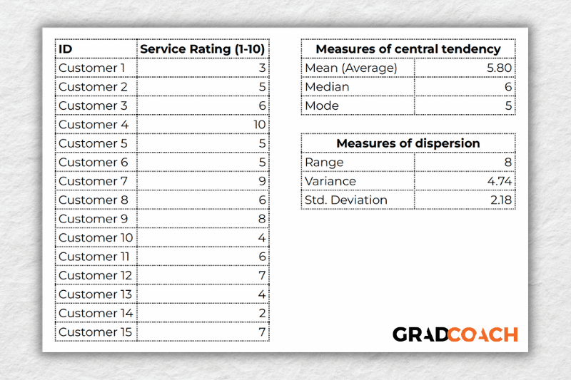
As you can see, the mean of 5.8 is the average rating across all 15 customers. Meanwhile, 6 is the median . In other words, if you were to list all the responses in order from low to high, Customer 8 would be in the middle (with their service rating being 6). Lastly, the number 5 is the most frequent rating (appearing 3 times), making it the mode.

Together, these three descriptive statistics give us a quick overview of how these customers feel about the service levels at this business. In other words, most customers feel rather lukewarm and there’s certainly room for improvement. From a more statistical perspective, this also means that the data tend to cluster around the 5-6 mark , since the mean and the median are fairly close to each other.

To take this a step further, let’s look at the frequency distribution of the responses . In other words, let’s count how many times each rating was received, and then plot these counts onto a bar chart.

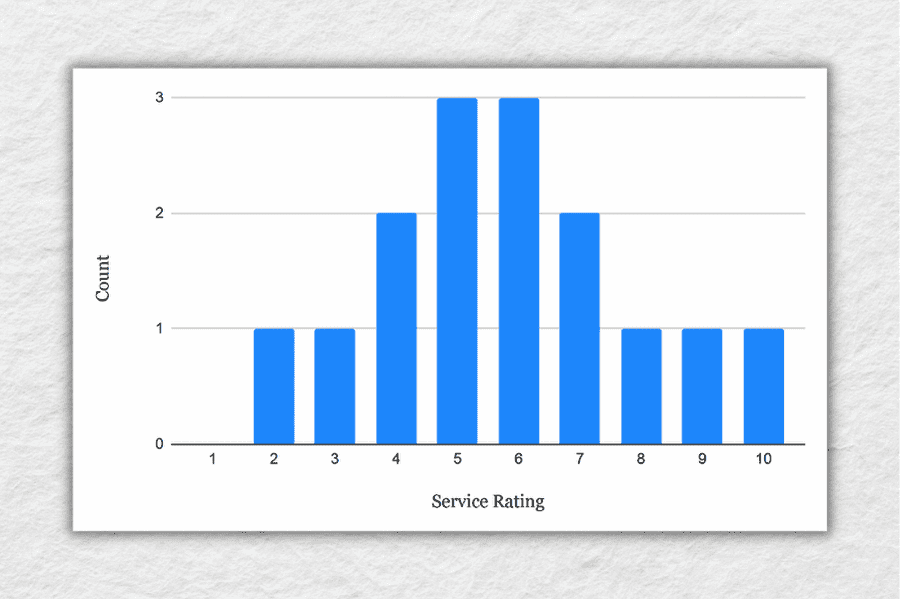
As you can see, the responses tend to cluster toward the centre of the chart , creating something of a bell-shaped curve. In statistical terms, this is called a normal distribution .

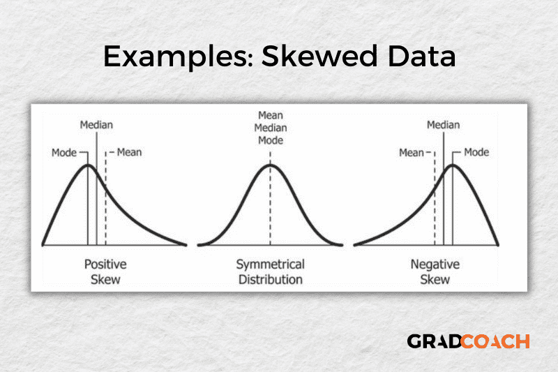
As you delve into quantitative data analysis, you’ll find that normal distributions are very common , but they’re certainly not the only type of distribution. In some cases, the data can lean toward the left or the right of the chart (i.e., toward the low end or high end). This lean is reflected by a measure called skewness , and it’s important to pay attention to this when you’re analysing your data, as this will have an impact on what types of inferential statistics you can use on your dataset.

Measures of dispersion

While the measures of central tendency provide insight into how “centred” the dataset is, it’s also important to understand how dispersed that dataset is . In other words, to what extent the data cluster toward the centre – specifically, the mean. In some cases, the majority of the data points will sit very close to the centre, while in other cases, they’ll be scattered all over the place. Enter the measures of dispersion, of which there are three:

Range , which measures the difference between the largest and smallest number in the dataset. In other words, it indicates how spread out the dataset really is.

Variance , which measures how much each number in a dataset varies from the mean (average). More technically, it calculates the average of the squared differences between each number and the mean. A higher variance indicates that the data points are more spread out , while a lower variance suggests that the data points are closer to the mean.

Standard deviation , which is the square root of the variance . It serves the same purposes as the variance, but is a bit easier to interpret as it presents a figure that is in the same unit as the original data . You’ll typically present this statistic alongside the means when describing the data in your research.

Again, let’s look at our sample dataset to make this all a little more tangible.

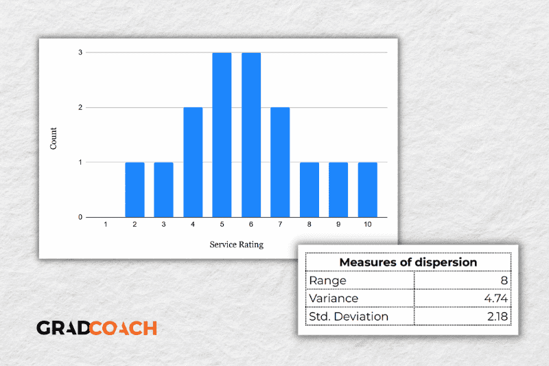
As you can see, the range of 8 reflects the difference between the highest rating (10) and the lowest rating (2). The standard deviation of 2.18 tells us that on average, results within the dataset are 2.18 away from the mean (of 5.8), reflecting a relatively dispersed set of data .

For the sake of comparison, let’s look at another much more tightly grouped (less dispersed) dataset.

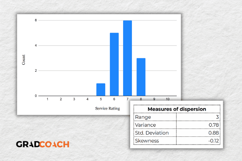
As you can see, all the ratings lay between 5 and 8 in this dataset, resulting in a much smaller range, variance and standard deviation . You might also notice that the data are clustered toward the right side of the graph – in other words, the data are skewed. If we calculate the skewness for this dataset, we get a result of -0.12, confirming this right lean.

In summary, range, variance and standard deviation all provide an indication of how dispersed the data are . These measures are important because they help you interpret the measures of central tendency within context . In other words, if your measures of dispersion are all fairly high numbers, you need to interpret your measures of central tendency with some caution , as the results are not particularly centred. Conversely, if the data are all tightly grouped around the mean (i.e., low dispersion), the mean becomes a much more “meaningful” statistic).

Key Takeaways

We’ve covered quite a bit of ground in this post. Here are the key takeaways:

• Descriptive statistics, although relatively simple, are a critically important part of any quantitative data analysis.
• Measures of central tendency include the mean (average), median and mode.
• Skewness indicates whether a dataset leans to one side or another
• Measures of dispersion include the range, variance and standard deviation

If you’d like hands-on help with your descriptive statistics (or any other aspect of your research project), check out our private coaching service , where we hold your hand through each step of the research journey.

Learn More About Methodology

How To Choose A Tutor For Your Dissertation

Hiring the right tutor for your dissertation or thesis can make the difference between passing and failing. Here’s what you need to consider.

5 Signs You Need A Dissertation Helper

Discover the 5 signs that suggest you need a dissertation helper to get unstuck, finish your degree and get your life back.

Triangulation: The Ultimate Credibility Enhancer

Triangulation is one of the best ways to enhance the credibility of your research. Learn about the different options here.

Research Limitations 101: What You Need To Know

Learn everything you need to know about research limitations (AKA limitations of the study). Includes practical examples from real studies.

In Vivo Coding 101: Full Explainer With Examples

Learn about in vivo coding, a popular qualitative coding technique ideal for studies where the nuances of language are central to the aims.

📄 FREE TEMPLATES

Research Topic Ideation

Proposal Writing

Literature Review

Methodology & Analysis

Academic Writing

Referencing & Citing

Apps, Tools & Tricks

The Grad Coach Podcast

Good day. May I ask about where I would be able to find the statistics cheat sheet?

Right above you comment 🙂

Good job. you saved me

Brilliant and well explained. So much information explained clearly!

Submit a Comment Cancel reply

Your email address will not be published. Required fields are marked *

Save my name, email, and website in this browser for the next time I comment.

Submit Comment

• Print Friendly

An official website of the United States government

Official websites use .gov A .gov website belongs to an official government organization in the United States.

Secure .gov websites use HTTPS A lock ( Lock Locked padlock icon ) or https:// means you've safely connected to the .gov website. Share sensitive information only on official, secure websites.

• Publications
• Account settings
• Advanced Search
• Journal List

Study designs: Part 2 – Descriptive studies

Rakesh aggarwal, priya ranganathan.

• Author information
• Copyright and License information

Address for correspondence: Dr. Rakesh Aggarwal, Department of Gastroenterology, Sanjay Gandhi Postgraduate Institute of Medical Sciences, Lucknow, Uttar Pradesh, India. E-mail: [email protected]

This is an open access journal, and articles are distributed under the terms of the Creative Commons Attribution-NonCommercial-ShareAlike 4.0 License, which allows others to remix, tweak, and build upon the work non-commercially, as long as appropriate credit is given and the new creations are licensed under the identical terms.

One of the first steps in planning a research study is the choice of study design. The available study designs are divided broadly into two types – observational and interventional. Of the various observational study designs, the descriptive design is the simplest. It allows the researcher to study and describe the distribution of one or more variables, without regard to any causal or other hypotheses. This article discusses the subtypes of descriptive study design, and their strengths and limitations.

Keywords: Epidemiologic methods, observational studies, research design

INTRODUCTION

In our previous article in this series,[ 1 ] we introduced the concept of “study designs”– as “the set of methods and procedures used to collect and analyze data on variables specified in a particular research question.” Study designs are primarily of two types – observational and interventional, with the former being loosely divided into “descriptive” and “analytical.” In this article, we discuss the descriptive study designs.

WHAT IS A DESCRIPTIVE STUDY?

A descriptive study is one that is designed to describe the distribution of one or more variables, without regard to any causal or other hypothesis.

TYPES OF DESCRIPTIVE STUDIES

Descriptive studies can be of several types, namely, case reports, case series, cross-sectional studies, and ecological studies. In the first three of these, data are collected on individuals, whereas the last one uses aggregated data for groups.

Case reports and case series

A case report refers to the description of a patient with an unusual disease or with simultaneous occurrence of more than one condition. A case series is similar, except that it is an aggregation of multiple (often only a few) similar cases. Many case reports and case series are anecdotal and of limited value. However, some of these bring to the fore a hitherto unrecognized disease and play an important role in advancing medical science. For instance, HIV/AIDS was first recognized through a case report of disseminated Kaposi's sarcoma in a young homosexual man,[ 2 ] and a case series of such men with Pneumocystis carinii pneumonia.[ 3 ]

In other cases, description of a chance observation may open an entirely new line of investigation. Some examples include: fatal disseminated Bacillus Calmette–Guérin infection in a baby born to a mother taking infliximab for Crohn's disease suggesting that adminstration of infliximab may bring about reactivation of tuberculosis,[ 4 ] progressive multifocal leukoencephalopathy following natalizumab treatment – describing a new adverse effect of drugs that target cell adhesion molecule α4-integrin,[ 5 ] and demonstration of a tumor caused by invasive transformed cancer cells from a colonizing tapeworm in an HIV-infected person.[ 6 ]

Cross-sectional studies

Studies with a cross-sectional study design involve the collection of information on the presence or level of one or more variables of interest (health-related characteristic), whether exposure (e.g., a risk factor) or outcome (e.g., a disease) as they exist in a defined population at one particular time. If these data are analyzed only to determine the distribution of one or more variables, these are “descriptive.” However, often, in a cross-sectional study, the investigator also assesses the relationship between the presence of an exposure and that of an outcome. Such cross-sectional studies are referred to as “analytical” and will be discussed in the next article in this series.

Cross-sectional studies can be thought of as providing a “snapshot” of the frequency and characteristics of a disease in a population at a particular point in time. These are very good for measuring the prevalence of a disease or of a risk factor in a population. Thus, these are very helpful in assessing the disease burden and healthcare needs.

Let us look at a study that was aimed to assess the prevalence of myopia among Indian children.[ 7 ] In this study, trained health workers visited schools in Delhi and tested visual acuity in all children studying in classes 1–9. Of the 9884 children screened, 1297 (13.1%) had myopia (defined as spherical refractive error of −0.50 diopters (D) or worse in either or both eyes), and the mean myopic error was −1.86 ± 1.4 D. Furthermore, overall, 322 (3.3%), 247 (2.5%) and 3 children had mild, moderate, and severe visual impairment, respectively. These parts of the study looked at the prevalence and degree of myopia or of visual impairment, and did not assess the relationship of one variable with another or test a causative hypothesis – these qualify as a descriptive cross-sectional study. These data would be helpful to a health planner to assess the need for a school eye health program, and to know the proportion of children in her jurisdiction who would need corrective glasses.

The authors did, subsequently in the paper, look at the relationship of myopia (an outcome) with children's age, gender, socioeconomic status, type of school, mother's education, etc. (each of which qualifies as an exposure). Those parts of the paper look at the relationship between different variables and thus qualify as having “analytical” cross-sectional design.

Sometimes, cross-sectional studies are repeated after a time interval in the same population (using the same subjects as were included in the initial study, or a fresh sample) to identify temporal trends in the occurrence of one or more variables, and to determine the incidence of a disease (i.e., number of new cases) or its natural history. Indeed, the investigators in the myopia study above visited the same children and reassessed them a year later. This separate follow-up study[ 8 ] showed that “new” myopia had developed in 3.4% of children (incidence rate), with a mean change of −1.09 ± 0.55 D. Among those with myopia at the time of the initial survey, 49.2% showed progression of myopia with a mean change of −0.27 ± 0.42 D.

Cross-sectional studies are usually simple to do and inexpensive. Furthermore, these usually do not pose much of a challenge from an ethics viewpoint.

However, this design does carry a risk of bias, i.e., the results of the study may not represent the true situation in the population. This could arise from either selection bias or measurement bias. The former relates to differences between the population and the sample studied. The myopia study included only those children who attended school, and the prevalence of myopia could have been different in those did not attend school (e.g., those with severe myopia may not be able to see the blackboard and hence may have been more likely to drop out of school). The measurement bias in this study would relate to the accuracy of measurement and the cutoff used. If the investigators had used a cutoff of −0.25 D (instead of −0.50 D) to define myopia, the prevalence would have been higher. Furthermore, if the measurements were not done accurately, some cases with myopia could have been missed, or vice versa, affecting the study results.

Ecological studies

Ecological (also sometimes called as correlational) study design involves looking for association between an exposure and an outcome across populations rather than in individuals. For instance, a study in the United States found a relation between household firearm ownership in various states and the firearm death rates during the period 2007–2010.[ 9 ] Thus, in this study, the unit of assessment was a state and not an individual.

These studies are convenient to do since the data have often already been collected and are available from a reliable source. This design is particularly useful when the differences in exposure between individuals within a group are much smaller than the differences in exposure between groups. For instance, the intake of particular food items is likely to vary less between people in a particular group but can vary widely across groups, for example, people living in different countries.

However, the ecological study design has some important limitations.First, an association between exposure and outcome at the group level may not be true at the individual level (a phenomenon also referred to as “ecological fallacy”).[ 10 ] Second, the association may be related to a third factor which in turn is related to both the exposure and the outcome, the so-called “confounding”. For instance, an ecological association between higher income level and greater cardiovascular mortality across countries may be related to a higher prevalence of obesity. Third, migration of people between regions with different exposure levels may also introduce an error. A fourth consideration may be the use of differing definitions for exposure, outcome or both in different populations.

Descriptive studies, irrespective of the subtype, are often very easy to conduct. For case reports, case series, and ecological studies, the data are already available. For cross-sectional studies, these can be easily collected (usually in one encounter). Thus, these study designs are often inexpensive, quick and do not need too much effort. Furthermore, these studies often do not face serious ethics scrutiny, except if the information sought to be collected is of confidential nature (e.g., sexual practices, substance use, etc.).

Descriptive studies are useful for estimating the burden of disease (e.g., prevalence or incidence) in a population. This information is useful for resource planning. For instance, information on prevalence of cataract in a city may help the government decide on the appropriate number of ophthalmologic facilities. Data from descriptive studies done in different populations or done at different times in the same population may help identify geographic variation and temporal change in the frequency of disease. This may help generate hypotheses regarding the cause of the disease, which can then be verified using another, more complex design.

DISADVANTAGES

As with other study designs, descriptive studies have their own pitfalls. Case reports and case-series refer to a solitary patient or to only a few cases, who may represent a chance occurrence. Hence, conclusions based on these run the risk of being non-representative, and hence unreliable. In cross-sectional studies, the validity of results is highly dependent on whether the study sample is well representative of the population proposed to be studied, and whether all the individual measurements were made using an accurate and identical tool, or not. If the information on a variable cannot be obtained accurately, for instance in a study where the participants are asked about socially unacceptable (e.g., promiscuity) or illegal (e.g., substance use) behavior, the results are unlikely to be reliable.

Financial support and sponsorship

Conflicts of interest.

There are no conflicts of interest.

• 1. Ranganathan P, Aggarwal R. Study designs: Part 1 – An overview and classification. Perspect Clin Res. 2018;9:184–6. doi: 10.4103/picr.PICR_124_18. [ DOI ] [ PMC free article ] [ PubMed ] [ Google Scholar ]
• 2. Gottlieb GJ, Ragaz A, Vogel JV, Friedman-Kien A, Rywlin AM, Weiner EA, et al. A preliminary communication on extensively disseminated Kaposi's sarcoma in young homosexual men. Am J Dermatopathol. 1981;3:111–4. doi: 10.1097/00000372-198100320-00002. [ DOI ] [ PubMed ] [ Google Scholar ]
• 3. Centers for Disease Control (CDC). Pneumocystis pneumonia – Los Angeles. MMWR Morb Mortal Wkly Rep. 30:250–2. [ PubMed ] [ Google Scholar ]
• 4. Cheent K, Nolan J, Shariq S, Kiho L, Pal A, Arnold J, et al. Case report: Fatal case of disseminated BCG infection in an infant born to a mother taking infliximab for Crohn's disease. J Crohns Colitis. 2010;4:603–5. doi: 10.1016/j.crohns.2010.05.001. [ DOI ] [ PubMed ] [ Google Scholar ]
• 5. Van Assche G, Van Ranst M, Sciot R, Dubois B, Vermeire S, Noman M, et al. Progressive multifocal leukoencephalopathy after natalizumab therapy for Crohn's disease. N Engl J Med. 2005;353:362–8. doi: 10.1056/NEJMoa051586. [ DOI ] [ PubMed ] [ Google Scholar ]
• 6. Muehlenbachs A, Bhatnagar J, Agudelo CA, Hidron A, Eberhard ML, Mathison BA, et al. Malignant transformation of Hymenolepis nana in a human host. N Engl J Med. 2015;373:1845–52. doi: 10.1056/NEJMoa1505892. [ DOI ] [ PubMed ] [ Google Scholar ]
• 7. Saxena R, Vashist P, Tandon R, Pandey RM, Bhardawaj A, Menon V, et al. Prevalence of myopia and its risk factors in urban school children in Delhi: The North India myopia study (NIM study) PLoS One. 2015;10:e0117349. doi: 10.1371/journal.pone.0117349. [ DOI ] [ PMC free article ] [ PubMed ] [ Google Scholar ]
• 8. Saxena R, Vashist P, Tandon R, Pandey RM, Bhardawaj A, Gupta V, et al. Incidence and progression of myopia and associated factors in urban school children in Delhi: The North India myopia study (NIM study) PLoS One. 2017;12:e0189774. doi: 10.1371/journal.pone.0189774. [ DOI ] [ PMC free article ] [ PubMed ] [ Google Scholar ]
• 9. Fleegler EW, Lee LK, Monuteaux MC, Hemenway D, Mannix R. Firearm legislation and firearm-related fatalities in the United States. JAMA Intern Med. 2013;173:732–40. doi: 10.1001/jamainternmed.2013.1286. [ DOI ] [ PubMed ] [ Google Scholar ]
• 10. Sedgwick P. Understanding the ecological fallacy. BMJ. 2015;351:h4773. doi: 10.1136/bmj.h4773. [ DOI ] [ PubMed ] [ Google Scholar ]
• View on publisher site
• PDF (389.8 KB)
• Collections

Similar articles

Cited by other articles, links to ncbi databases.

• Download .nbib .nbib
• Format: AMA APA MLA NLM

Add to Collections

Want to create or adapt books like this? Learn more about how Pressbooks supports open publishing practices.

14 Quantitative analysis: Descriptive statistics

Numeric data collected in a research project can be analysed quantitatively using statistical tools in two different ways. Descriptive analysis refers to statistically describing, aggregating, and presenting the constructs of interest or associations between these constructs. Inferential analysis refers to the statistical testing of hypotheses (theory testing). In this chapter, we will examine statistical techniques used for descriptive analysis, and the next chapter will examine statistical techniques for inferential analysis. Much of today’s quantitative data analysis is conducted using software programs such as SPSS or SAS. Readers are advised to familiarise themselves with one of these programs for understanding the concepts described in this chapter.

Data preparation

In research projects, data may be collected from a variety of sources: postal surveys, interviews, pretest or posttest experimental data, observational data, and so forth. This data must be converted into a machine-readable, numeric format, such as in a spreadsheet or a text file, so that they can be analysed by computer programs like SPSS or SAS. Data preparation usually follows the following steps:

Data coding. Coding is the process of converting data into numeric format. A codebook should be created to guide the coding process. A codebook is a comprehensive document containing a detailed description of each variable in a research study, items or measures for that variable, the format of each item (numeric, text, etc.), the response scale for each item (i.e., whether it is measured on a nominal, ordinal, interval, or ratio scale, and whether this scale is a five-point, seven-point scale, etc.), and how to code each value into a numeric format. For instance, if we have a measurement item on a seven-point Likert scale with anchors ranging from ‘strongly disagree’ to ‘strongly agree’, we may code that item as 1 for strongly disagree, 4 for neutral, and 7 for strongly agree, with the intermediate anchors in between. Nominal data such as industry type can be coded in numeric form using a coding scheme such as: 1 for manufacturing, 2 for retailing, 3 for financial, 4 for healthcare, and so forth (of course, nominal data cannot be analysed statistically). Ratio scale data such as age, income, or test scores can be coded as entered by the respondent. Sometimes, data may need to be aggregated into a different form than the format used for data collection. For instance, if a survey measuring a construct such as ‘benefits of computers’ provided respondents with a checklist of benefits that they could select from, and respondents were encouraged to choose as many of those benefits as they wanted, then the total number of checked items could be used as an aggregate measure of benefits. Note that many other forms of data—such as interview transcripts—cannot be converted into a numeric format for statistical analysis. Codebooks are especially important for large complex studies involving many variables and measurement items, where the coding process is conducted by different people, to help the coding team code data in a consistent manner, and also to help others understand and interpret the coded data.

Data entry. Coded data can be entered into a spreadsheet, database, text file, or directly into a statistical program like SPSS. Most statistical programs provide a data editor for entering data. However, these programs store data in their own native format—e.g., SPSS stores data as .sav files—which makes it difficult to share that data with other statistical programs. Hence, it is often better to enter data into a spreadsheet or database where it can be reorganised as needed, shared across programs, and subsets of data can be extracted for analysis. Smaller data sets with less than 65,000 observations and 256 items can be stored in a spreadsheet created using a program such as Microsoft Excel, while larger datasets with millions of observations will require a database. Each observation can be entered as one row in the spreadsheet, and each measurement item can be represented as one column. Data should be checked for accuracy during and after entry via occasional spot checks on a set of items or observations. Furthermore, while entering data, the coder should watch out for obvious evidence of bad data, such as the respondent selecting the ‘strongly agree’ response to all items irrespective of content, including reverse-coded items. If so, such data can be entered but should be excluded from subsequent analysis.

Data transformation. Sometimes, it is necessary to transform data values before they can be meaningfully interpreted. For instance, reverse coded items—where items convey the opposite meaning of that of their underlying construct—should be reversed (e.g., in a 1-7 interval scale, 8 minus the observed value will reverse the value) before they can be compared or combined with items that are not reverse coded. Other kinds of transformations may include creating scale measures by adding individual scale items, creating a weighted index from a set of observed measures, and collapsing multiple values into fewer categories (e.g., collapsing incomes into income ranges).

Univariate analysis

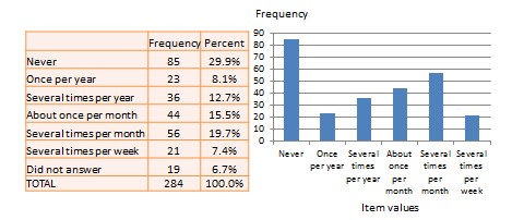
Univariate analysis—or analysis of a single variable—refers to a set of statistical techniques that can describe the general properties of one variable. Univariate statistics include: frequency distribution, central tendency, and dispersion. The frequency distribution of a variable is a summary of the frequency—or percentages—of individual values or ranges of values for that variable. For instance, we can measure how many times a sample of respondents attend religious services—as a gauge of their ‘religiosity’—using a categorical scale: never, once per year, several times per year, about once a month, several times per month, several times per week, and an optional category for ‘did not answer’. If we count the number or percentage of observations within each category—except ‘did not answer’ which is really a missing value rather than a category—and display it in the form of a table, as shown in Figure 14.1, what we have is a frequency distribution. This distribution can also be depicted in the form of a bar chart, as shown on the right panel of Figure 14.1, with the horizontal axis representing each category of that variable and the vertical axis representing the frequency or percentage of observations within each category.

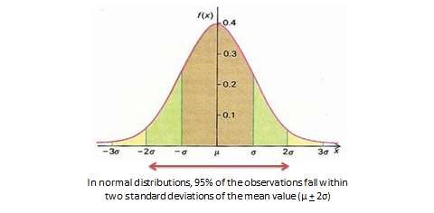
With very large samples, where observations are independent and random, the frequency distribution tends to follow a plot that looks like a bell-shaped curve—a smoothed bar chart of the frequency distribution—similar to that shown in Figure 14.2. Here most observations are clustered toward the centre of the range of values, with fewer and fewer observations clustered toward the extreme ends of the range. Such a curve is called a normal distribution .

Lastly, the mode is the most frequently occurring value in a distribution of values. In the previous example, the most frequently occurring value is 15, which is the mode of the above set of test scores. Note that any value that is estimated from a sample, such as mean, median, mode, or any of the later estimates are called a statistic .

Bivariate analysis

Bivariate analysis examines how two variables are related to one another. The most common bivariate statistic is the bivariate correlation —often, simply called ‘correlation’—which is a number between -1 and +1 denoting the strength of the relationship between two variables. Say that we wish to study how age is related to self-esteem in a sample of 20 respondents—i.e., as age increases, does self-esteem increase, decrease, or remain unchanged?. If self-esteem increases, then we have a positive correlation between the two variables, if self-esteem decreases, then we have a negative correlation, and if it remains the same, we have a zero correlation. To calculate the value of this correlation, consider the hypothetical dataset shown in Table 14.1.

After computing bivariate correlation, researchers are often interested in knowing whether the correlation is significant (i.e., a real one) or caused by mere chance. Answering such a question would require testing the following hypothesis:

Social Science Research: Principles, Methods and Practices (Revised edition) Copyright © 2019 by Anol Bhattacherjee is licensed under a Creative Commons Attribution-NonCommercial-ShareAlike 4.0 International License , except where otherwise noted.

Share This Book