Have a language expert improve your writing
Run a free plagiarism check in 10 minutes, generate accurate citations for free.
- Knowledge Base
Methodology
- Quasi-Experimental Design | Definition, Types & Examples

Quasi-Experimental Design | Definition, Types & Examples
Published on July 31, 2020 by Lauren Thomas . Revised on January 22, 2024.
Like a true experiment , a quasi-experimental design aims to establish a cause-and-effect relationship between an independent and dependent variable .
However, unlike a true experiment, a quasi-experiment does not rely on random assignment . Instead, subjects are assigned to groups based on non-random criteria.
Quasi-experimental design is a useful tool in situations where true experiments cannot be used for ethical or practical reasons.

Table of contents
Differences between quasi-experiments and true experiments, types of quasi-experimental designs, when to use quasi-experimental design, advantages and disadvantages, other interesting articles, frequently asked questions about quasi-experimental designs.
There are several common differences between true and quasi-experimental designs.
| True experimental design | Quasi-experimental design | |
|---|---|---|
| Assignment to treatment | The researcher subjects to control and treatment groups. | Some other, method is used to assign subjects to groups. |
| Control over treatment | The researcher usually . | The researcher often , but instead studies pre-existing groups that received different treatments after the fact. |
| Use of | Requires the use of . | Control groups are not required (although they are commonly used). |
Example of a true experiment vs a quasi-experiment
However, for ethical reasons, the directors of the mental health clinic may not give you permission to randomly assign their patients to treatments. In this case, you cannot run a true experiment.
Instead, you can use a quasi-experimental design.
You can use these pre-existing groups to study the symptom progression of the patients treated with the new therapy versus those receiving the standard course of treatment.
Receive feedback on language, structure, and formatting
Professional editors proofread and edit your paper by focusing on:
- Academic style
- Vague sentences
- Style consistency
See an example

Many types of quasi-experimental designs exist. Here we explain three of the most common types: nonequivalent groups design, regression discontinuity, and natural experiments.
Nonequivalent groups design
In nonequivalent group design, the researcher chooses existing groups that appear similar, but where only one of the groups experiences the treatment.
In a true experiment with random assignment , the control and treatment groups are considered equivalent in every way other than the treatment. But in a quasi-experiment where the groups are not random, they may differ in other ways—they are nonequivalent groups .
When using this kind of design, researchers try to account for any confounding variables by controlling for them in their analysis or by choosing groups that are as similar as possible.
This is the most common type of quasi-experimental design.
Regression discontinuity
Many potential treatments that researchers wish to study are designed around an essentially arbitrary cutoff, where those above the threshold receive the treatment and those below it do not.
Near this threshold, the differences between the two groups are often so minimal as to be nearly nonexistent. Therefore, researchers can use individuals just below the threshold as a control group and those just above as a treatment group.
However, since the exact cutoff score is arbitrary, the students near the threshold—those who just barely pass the exam and those who fail by a very small margin—tend to be very similar, with the small differences in their scores mostly due to random chance. You can therefore conclude that any outcome differences must come from the school they attended.
Natural experiments
In both laboratory and field experiments, researchers normally control which group the subjects are assigned to. In a natural experiment, an external event or situation (“nature”) results in the random or random-like assignment of subjects to the treatment group.
Even though some use random assignments, natural experiments are not considered to be true experiments because they are observational in nature.
Although the researchers have no control over the independent variable , they can exploit this event after the fact to study the effect of the treatment.
However, as they could not afford to cover everyone who they deemed eligible for the program, they instead allocated spots in the program based on a random lottery.
Although true experiments have higher internal validity , you might choose to use a quasi-experimental design for ethical or practical reasons.
Sometimes it would be unethical to provide or withhold a treatment on a random basis, so a true experiment is not feasible. In this case, a quasi-experiment can allow you to study the same causal relationship without the ethical issues.
The Oregon Health Study is a good example. It would be unethical to randomly provide some people with health insurance but purposely prevent others from receiving it solely for the purposes of research.
However, since the Oregon government faced financial constraints and decided to provide health insurance via lottery, studying this event after the fact is a much more ethical approach to studying the same problem.
True experimental design may be infeasible to implement or simply too expensive, particularly for researchers without access to large funding streams.
At other times, too much work is involved in recruiting and properly designing an experimental intervention for an adequate number of subjects to justify a true experiment.
In either case, quasi-experimental designs allow you to study the question by taking advantage of data that has previously been paid for or collected by others (often the government).
Quasi-experimental designs have various pros and cons compared to other types of studies.
- Higher external validity than most true experiments, because they often involve real-world interventions instead of artificial laboratory settings.
- Higher internal validity than other non-experimental types of research, because they allow you to better control for confounding variables than other types of studies do.
- Lower internal validity than true experiments—without randomization, it can be difficult to verify that all confounding variables have been accounted for.
- The use of retrospective data that has already been collected for other purposes can be inaccurate, incomplete or difficult to access.
Here's why students love Scribbr's proofreading services
Discover proofreading & editing
If you want to know more about statistics , methodology , or research bias , make sure to check out some of our other articles with explanations and examples.
- Normal distribution
- Degrees of freedom
- Null hypothesis
- Discourse analysis
- Control groups
- Mixed methods research
- Non-probability sampling
- Quantitative research
- Ecological validity
Research bias
- Rosenthal effect
- Implicit bias
- Cognitive bias
- Selection bias
- Negativity bias
- Status quo bias
A quasi-experiment is a type of research design that attempts to establish a cause-and-effect relationship. The main difference with a true experiment is that the groups are not randomly assigned.
In experimental research, random assignment is a way of placing participants from your sample into different groups using randomization. With this method, every member of the sample has a known or equal chance of being placed in a control group or an experimental group.
Quasi-experimental design is most useful in situations where it would be unethical or impractical to run a true experiment .
Quasi-experiments have lower internal validity than true experiments, but they often have higher external validity as they can use real-world interventions instead of artificial laboratory settings.
Cite this Scribbr article
If you want to cite this source, you can copy and paste the citation or click the “Cite this Scribbr article” button to automatically add the citation to our free Citation Generator.
Thomas, L. (2024, January 22). Quasi-Experimental Design | Definition, Types & Examples. Scribbr. Retrieved September 9, 2024, from https://www.scribbr.com/methodology/quasi-experimental-design/
Is this article helpful?

Lauren Thomas
Other students also liked, guide to experimental design | overview, steps, & examples, random assignment in experiments | introduction & examples, control variables | what are they & why do they matter, "i thought ai proofreading was useless but..".
I've been using Scribbr for years now and I know it's a service that won't disappoint. It does a good job spotting mistakes”
- Skip to secondary menu
- Skip to main content
- Skip to primary sidebar
Statistics By Jim
Making statistics intuitive
Quasi Experimental Design Overview & Examples
By Jim Frost Leave a Comment
What is a Quasi Experimental Design?
A quasi experimental design is a method for identifying causal relationships that does not randomly assign participants to the experimental groups. Instead, researchers use a non-random process. For example, they might use an eligibility cutoff score or preexisting groups to determine who receives the treatment.

Quasi-experimental research is a design that closely resembles experimental research but is different. The term “quasi” means “resembling,” so you can think of it as a cousin to actual experiments. In these studies, researchers can manipulate an independent variable — that is, they change one factor to see what effect it has. However, unlike true experimental research, participants are not randomly assigned to different groups.
Learn more about Experimental Designs: Definition & Types .
When to Use Quasi-Experimental Design
Researchers typically use a quasi-experimental design because they can’t randomize due to practical or ethical concerns. For example:
- Practical Constraints : A school interested in testing a new teaching method can only implement it in preexisting classes and cannot randomly assign students.
- Ethical Concerns : A medical study might not be able to randomly assign participants to a treatment group for an experimental medication when they are already taking a proven drug.
Quasi-experimental designs also come in handy when researchers want to study the effects of naturally occurring events, like policy changes or environmental shifts, where they can’t control who is exposed to the treatment.
Quasi-experimental designs occupy a unique position in the spectrum of research methodologies, sitting between observational studies and true experiments. This middle ground offers a blend of both worlds, addressing some limitations of purely observational studies while navigating the constraints often accompanying true experiments.
A significant advantage of quasi-experimental research over purely observational studies and correlational research is that it addresses the issue of directionality, determining which variable is the cause and which is the effect. In quasi-experiments, an intervention typically occurs during the investigation, and the researchers record outcomes before and after it, increasing the confidence that it causes the observed changes.
However, it’s crucial to recognize its limitations as well. Controlling confounding variables is a larger concern for a quasi-experimental design than a true experiment because it lacks random assignment.
In sum, quasi-experimental designs offer a valuable research approach when random assignment is not feasible, providing a more structured and controlled framework than observational studies while acknowledging and attempting to address potential confounders.
Types of Quasi-Experimental Designs and Examples
Quasi-experimental studies use various methods, depending on the scenario.
Natural Experiments
This design uses naturally occurring events or changes to create the treatment and control groups. Researchers compare outcomes between those whom the event affected and those it did not affect. Analysts use statistical controls to account for confounders that the researchers must also measure.
Natural experiments are related to observational studies, but they allow for a clearer causality inference because the external event or policy change provides both a form of quasi-random group assignment and a definite start date for the intervention.
For example, in a natural experiment utilizing a quasi-experimental design, researchers study the impact of a significant economic policy change on small business growth. The policy is implemented in one state but not in neighboring states. This scenario creates an unplanned experimental setup, where the state with the new policy serves as the treatment group, and the neighboring states act as the control group.
Researchers are primarily interested in small business growth rates but need to record various confounders that can impact growth rates. Hence, they record state economic indicators, investment levels, and employment figures. By recording these metrics across the states, they can include them in the model as covariates and control them statistically. This method allows researchers to estimate differences in small business growth due to the policy itself, separate from the various confounders.
Nonequivalent Groups Design
This method involves matching existing groups that are similar but not identical. Researchers attempt to find groups that are as equivalent as possible, particularly for factors likely to affect the outcome.
For instance, researchers use a nonequivalent groups quasi-experimental design to evaluate the effectiveness of a new teaching method in improving students’ mathematics performance. A school district considering the teaching method is planning the study. Students are already divided into schools, preventing random assignment.
The researchers matched two schools with similar demographics, baseline academic performance, and resources. The school using the traditional methodology is the control, while the other uses the new approach. Researchers are evaluating differences in educational outcomes between the two methods.
They perform a pretest to identify differences between the schools that might affect the outcome and include them as covariates to control for confounding. They also record outcomes before and after the intervention to have a larger context for the changes they observe.
Regression Discontinuity
This process assigns subjects to a treatment or control group based on a predetermined cutoff point (e.g., a test score). The analysis primarily focuses on participants near the cutoff point, as they are likely similar except for the treatment received. By comparing participants just above and below the cutoff, the design controls for confounders that vary smoothly around the cutoff.
For example, in a regression discontinuity quasi-experimental design focusing on a new medical treatment for depression, researchers use depression scores as the cutoff point. Individuals with depression scores just above a certain threshold are assigned to receive the latest treatment, while those just below the threshold do not receive it. This method creates two closely matched groups: one that barely qualifies for treatment and one that barely misses out.
By comparing the mental health outcomes of these two groups over time, researchers can assess the effectiveness of the new treatment. The assumption is that the only significant difference between the groups is whether they received the treatment, thereby isolating its impact on depression outcomes.
Controlling Confounders in a Quasi-Experimental Design
Accounting for confounding variables is a challenging but essential task for a quasi-experimental design.
In a true experiment, the random assignment process equalizes confounders across the groups to nullify their overall effect. It’s the gold standard because it works on all confounders, known and unknown.
Unfortunately, the lack of random assignment can allow differences between the groups to exist before the intervention. These confounding factors might ultimately explain the results rather than the intervention.
Consequently, researchers must use other methods to equalize the groups roughly using matching and cutoff values or statistically adjust for preexisting differences they measure to reduce the impact of confounders.
A key strength of quasi-experiments is their frequent use of “pre-post testing.” This approach involves conducting initial tests before collecting data to check for preexisting differences between groups that could impact the study’s outcome. By identifying these variables early on and including them as covariates, researchers can more effectively control potential confounders in their statistical analysis.
Additionally, researchers frequently track outcomes before and after the intervention to better understand the context for changes they observe.
Statisticians consider these methods to be less effective than randomization. Hence, quasi-experiments fall somewhere in the middle when it comes to internal validity , or how well the study can identify causal relationships versus mere correlation . They’re more conclusive than correlational studies but not as solid as true experiments.
In conclusion, quasi-experimental designs offer researchers a versatile and practical approach when random assignment is not feasible. This methodology bridges the gap between controlled experiments and observational studies, providing a valuable tool for investigating cause-and-effect relationships in real-world settings. Researchers can address ethical and logistical constraints by understanding and leveraging the different types of quasi-experimental designs while still obtaining insightful and meaningful results.
Cook, T. D., & Campbell, D. T. (1979). Quasi-experimentation: Design & analysis issues in field settings . Boston, MA: Houghton Mifflin
Share this:

Reader Interactions
Comments and questions cancel reply.
- Privacy Policy
Home » Quasi-Experimental Research Design – Types, Methods
Quasi-Experimental Research Design – Types, Methods
Table of Contents

Quasi-Experimental Design
Quasi-experimental design is a research method that seeks to evaluate the causal relationships between variables, but without the full control over the independent variable(s) that is available in a true experimental design.
In a quasi-experimental design, the researcher uses an existing group of participants that is not randomly assigned to the experimental and control groups. Instead, the groups are selected based on pre-existing characteristics or conditions, such as age, gender, or the presence of a certain medical condition.
Types of Quasi-Experimental Design
There are several types of quasi-experimental designs that researchers use to study causal relationships between variables. Here are some of the most common types:
Non-Equivalent Control Group Design
This design involves selecting two groups of participants that are similar in every way except for the independent variable(s) that the researcher is testing. One group receives the treatment or intervention being studied, while the other group does not. The two groups are then compared to see if there are any significant differences in the outcomes.
Interrupted Time-Series Design
This design involves collecting data on the dependent variable(s) over a period of time, both before and after an intervention or event. The researcher can then determine whether there was a significant change in the dependent variable(s) following the intervention or event.
Pretest-Posttest Design
This design involves measuring the dependent variable(s) before and after an intervention or event, but without a control group. This design can be useful for determining whether the intervention or event had an effect, but it does not allow for control over other factors that may have influenced the outcomes.
Regression Discontinuity Design
This design involves selecting participants based on a specific cutoff point on a continuous variable, such as a test score. Participants on either side of the cutoff point are then compared to determine whether the intervention or event had an effect.
Natural Experiments
This design involves studying the effects of an intervention or event that occurs naturally, without the researcher’s intervention. For example, a researcher might study the effects of a new law or policy that affects certain groups of people. This design is useful when true experiments are not feasible or ethical.
Data Analysis Methods
Here are some data analysis methods that are commonly used in quasi-experimental designs:
Descriptive Statistics
This method involves summarizing the data collected during a study using measures such as mean, median, mode, range, and standard deviation. Descriptive statistics can help researchers identify trends or patterns in the data, and can also be useful for identifying outliers or anomalies.
Inferential Statistics
This method involves using statistical tests to determine whether the results of a study are statistically significant. Inferential statistics can help researchers make generalizations about a population based on the sample data collected during the study. Common statistical tests used in quasi-experimental designs include t-tests, ANOVA, and regression analysis.
Propensity Score Matching
This method is used to reduce bias in quasi-experimental designs by matching participants in the intervention group with participants in the control group who have similar characteristics. This can help to reduce the impact of confounding variables that may affect the study’s results.
Difference-in-differences Analysis
This method is used to compare the difference in outcomes between two groups over time. Researchers can use this method to determine whether a particular intervention has had an impact on the target population over time.
Interrupted Time Series Analysis
This method is used to examine the impact of an intervention or treatment over time by comparing data collected before and after the intervention or treatment. This method can help researchers determine whether an intervention had a significant impact on the target population.
Regression Discontinuity Analysis
This method is used to compare the outcomes of participants who fall on either side of a predetermined cutoff point. This method can help researchers determine whether an intervention had a significant impact on the target population.
Steps in Quasi-Experimental Design
Here are the general steps involved in conducting a quasi-experimental design:
- Identify the research question: Determine the research question and the variables that will be investigated.
- Choose the design: Choose the appropriate quasi-experimental design to address the research question. Examples include the pretest-posttest design, non-equivalent control group design, regression discontinuity design, and interrupted time series design.
- Select the participants: Select the participants who will be included in the study. Participants should be selected based on specific criteria relevant to the research question.
- Measure the variables: Measure the variables that are relevant to the research question. This may involve using surveys, questionnaires, tests, or other measures.
- Implement the intervention or treatment: Implement the intervention or treatment to the participants in the intervention group. This may involve training, education, counseling, or other interventions.
- Collect data: Collect data on the dependent variable(s) before and after the intervention. Data collection may also include collecting data on other variables that may impact the dependent variable(s).
- Analyze the data: Analyze the data collected to determine whether the intervention had a significant impact on the dependent variable(s).
- Draw conclusions: Draw conclusions about the relationship between the independent and dependent variables. If the results suggest a causal relationship, then appropriate recommendations may be made based on the findings.
Quasi-Experimental Design Examples
Here are some examples of real-time quasi-experimental designs:
- Evaluating the impact of a new teaching method: In this study, a group of students are taught using a new teaching method, while another group is taught using the traditional method. The test scores of both groups are compared before and after the intervention to determine whether the new teaching method had a significant impact on student performance.
- Assessing the effectiveness of a public health campaign: In this study, a public health campaign is launched to promote healthy eating habits among a targeted population. The behavior of the population is compared before and after the campaign to determine whether the intervention had a significant impact on the target behavior.
- Examining the impact of a new medication: In this study, a group of patients is given a new medication, while another group is given a placebo. The outcomes of both groups are compared to determine whether the new medication had a significant impact on the targeted health condition.
- Evaluating the effectiveness of a job training program : In this study, a group of unemployed individuals is enrolled in a job training program, while another group is not enrolled in any program. The employment rates of both groups are compared before and after the intervention to determine whether the training program had a significant impact on the employment rates of the participants.
- Assessing the impact of a new policy : In this study, a new policy is implemented in a particular area, while another area does not have the new policy. The outcomes of both areas are compared before and after the intervention to determine whether the new policy had a significant impact on the targeted behavior or outcome.
Applications of Quasi-Experimental Design
Here are some applications of quasi-experimental design:
- Educational research: Quasi-experimental designs are used to evaluate the effectiveness of educational interventions, such as new teaching methods, technology-based learning, or educational policies.
- Health research: Quasi-experimental designs are used to evaluate the effectiveness of health interventions, such as new medications, public health campaigns, or health policies.
- Social science research: Quasi-experimental designs are used to investigate the impact of social interventions, such as job training programs, welfare policies, or criminal justice programs.
- Business research: Quasi-experimental designs are used to evaluate the impact of business interventions, such as marketing campaigns, new products, or pricing strategies.
- Environmental research: Quasi-experimental designs are used to evaluate the impact of environmental interventions, such as conservation programs, pollution control policies, or renewable energy initiatives.
When to use Quasi-Experimental Design
Here are some situations where quasi-experimental designs may be appropriate:
- When the research question involves investigating the effectiveness of an intervention, policy, or program : In situations where it is not feasible or ethical to randomly assign participants to intervention and control groups, quasi-experimental designs can be used to evaluate the impact of the intervention on the targeted outcome.
- When the sample size is small: In situations where the sample size is small, it may be difficult to randomly assign participants to intervention and control groups. Quasi-experimental designs can be used to investigate the impact of an intervention without requiring a large sample size.
- When the research question involves investigating a naturally occurring event : In some situations, researchers may be interested in investigating the impact of a naturally occurring event, such as a natural disaster or a major policy change. Quasi-experimental designs can be used to evaluate the impact of the event on the targeted outcome.
- When the research question involves investigating a long-term intervention: In situations where the intervention or program is long-term, it may be difficult to randomly assign participants to intervention and control groups for the entire duration of the intervention. Quasi-experimental designs can be used to evaluate the impact of the intervention over time.
- When the research question involves investigating the impact of a variable that cannot be manipulated : In some situations, it may not be possible or ethical to manipulate a variable of interest. Quasi-experimental designs can be used to investigate the relationship between the variable and the targeted outcome.
Purpose of Quasi-Experimental Design
The purpose of quasi-experimental design is to investigate the causal relationship between two or more variables when it is not feasible or ethical to conduct a randomized controlled trial (RCT). Quasi-experimental designs attempt to emulate the randomized control trial by mimicking the control group and the intervention group as much as possible.
The key purpose of quasi-experimental design is to evaluate the impact of an intervention, policy, or program on a targeted outcome while controlling for potential confounding factors that may affect the outcome. Quasi-experimental designs aim to answer questions such as: Did the intervention cause the change in the outcome? Would the outcome have changed without the intervention? And was the intervention effective in achieving its intended goals?
Quasi-experimental designs are useful in situations where randomized controlled trials are not feasible or ethical. They provide researchers with an alternative method to evaluate the effectiveness of interventions, policies, and programs in real-life settings. Quasi-experimental designs can also help inform policy and practice by providing valuable insights into the causal relationships between variables.
Overall, the purpose of quasi-experimental design is to provide a rigorous method for evaluating the impact of interventions, policies, and programs while controlling for potential confounding factors that may affect the outcome.
Advantages of Quasi-Experimental Design
Quasi-experimental designs have several advantages over other research designs, such as:
- Greater external validity : Quasi-experimental designs are more likely to have greater external validity than laboratory experiments because they are conducted in naturalistic settings. This means that the results are more likely to generalize to real-world situations.
- Ethical considerations: Quasi-experimental designs often involve naturally occurring events, such as natural disasters or policy changes. This means that researchers do not need to manipulate variables, which can raise ethical concerns.
- More practical: Quasi-experimental designs are often more practical than experimental designs because they are less expensive and easier to conduct. They can also be used to evaluate programs or policies that have already been implemented, which can save time and resources.
- No random assignment: Quasi-experimental designs do not require random assignment, which can be difficult or impossible in some cases, such as when studying the effects of a natural disaster. This means that researchers can still make causal inferences, although they must use statistical techniques to control for potential confounding variables.
- Greater generalizability : Quasi-experimental designs are often more generalizable than experimental designs because they include a wider range of participants and conditions. This can make the results more applicable to different populations and settings.
Limitations of Quasi-Experimental Design
There are several limitations associated with quasi-experimental designs, which include:
- Lack of Randomization: Quasi-experimental designs do not involve randomization of participants into groups, which means that the groups being studied may differ in important ways that could affect the outcome of the study. This can lead to problems with internal validity and limit the ability to make causal inferences.
- Selection Bias: Quasi-experimental designs may suffer from selection bias because participants are not randomly assigned to groups. Participants may self-select into groups or be assigned based on pre-existing characteristics, which may introduce bias into the study.
- History and Maturation: Quasi-experimental designs are susceptible to history and maturation effects, where the passage of time or other events may influence the outcome of the study.
- Lack of Control: Quasi-experimental designs may lack control over extraneous variables that could influence the outcome of the study. This can limit the ability to draw causal inferences from the study.
- Limited Generalizability: Quasi-experimental designs may have limited generalizability because the results may only apply to the specific population and context being studied.
About the author

Muhammad Hassan
Researcher, Academic Writer, Web developer
You may also like

Exploratory Research – Types, Methods and...

Focus Groups – Steps, Examples and Guide

Research Methods – Types, Examples and Guide

Observational Research – Methods and Guide

Experimental Design – Types, Methods, Guide

Correlational Research – Methods, Types and...
Our systems are now restored following recent technical disruption, and we’re working hard to catch up on publishing. We apologise for the inconvenience caused. Find out more: https://www.cambridge.org/universitypress/about-us/news-and-blogs/cambridge-university-press-publishing-update-following-technical-disruption
We use cookies to distinguish you from other users and to provide you with a better experience on our websites. Close this message to accept cookies or find out how to manage your cookie settings .
Login Alert
- > The Cambridge Handbook of Research Methods and Statistics for the Social and Behavioral Sciences
- > Quasi-Experimental Research

Book contents
- The Cambridge Handbook of Research Methods and Statistics for the Social and Behavioral Sciences
- Cambridge Handbooks in Psychology
- Copyright page
- Contributors
- Part I From Idea to Reality: The Basics of Research
- Part II The Building Blocks of a Study
- Part III Data Collection
- 13 Cross-Sectional Studies
- 14 Quasi-Experimental Research
- 15 Non-equivalent Control Group Pretest–Posttest Design in Social and Behavioral Research
- 16 Experimental Methods
- 17 Longitudinal Research: A World to Explore
- 18 Online Research Methods
- 19 Archival Data
- 20 Qualitative Research Design
- Part IV Statistical Approaches
- Part V Tips for a Successful Research Career
14 - Quasi-Experimental Research
from Part III - Data Collection
Published online by Cambridge University Press: 25 May 2023
In this chapter, we discuss the logic and practice of quasi-experimentation. Specifically, we describe four quasi-experimental designs – one-group pretest–posttest designs, non-equivalent group designs, regression discontinuity designs, and interrupted time-series designs – and their statistical analyses in detail. Both simple quasi-experimental designs and embellishments of these simple designs are presented. Potential threats to internal validity are illustrated along with means of addressing their potentially biasing effects so that these effects can be minimized. In contrast to quasi-experiments, randomized experiments are often thought to be the gold standard when estimating the effects of treatment interventions. However, circumstances frequently arise where quasi-experiments can usefully supplement randomized experiments or when quasi-experiments can fruitfully be used in place of randomized experiments. Researchers need to appreciate the relative strengths and weaknesses of the various quasi-experiments so they can choose among pre-specified designs or craft their own unique quasi-experiments.
Access options
Save book to kindle.
To save this book to your Kindle, first ensure [email protected] is added to your Approved Personal Document E-mail List under your Personal Document Settings on the Manage Your Content and Devices page of your Amazon account. Then enter the ‘name’ part of your Kindle email address below. Find out more about saving to your Kindle .
Note you can select to save to either the @free.kindle.com or @kindle.com variations. ‘@free.kindle.com’ emails are free but can only be saved to your device when it is connected to wi-fi. ‘@kindle.com’ emails can be delivered even when you are not connected to wi-fi, but note that service fees apply.
Find out more about the Kindle Personal Document Service .
- Quasi-Experimental Research
- By Charles S. Reichardt , Daniel Storage , Damon Abraham
- Edited by Austin Lee Nichols , Central European University, Vienna , John Edlund , Rochester Institute of Technology, New York
- Book: The Cambridge Handbook of Research Methods and Statistics for the Social and Behavioral Sciences
- Online publication: 25 May 2023
- Chapter DOI: https://doi.org/10.1017/9781009010054.015
Save book to Dropbox
To save content items to your account, please confirm that you agree to abide by our usage policies. If this is the first time you use this feature, you will be asked to authorise Cambridge Core to connect with your account. Find out more about saving content to Dropbox .
Save book to Google Drive
To save content items to your account, please confirm that you agree to abide by our usage policies. If this is the first time you use this feature, you will be asked to authorise Cambridge Core to connect with your account. Find out more about saving content to Google Drive .
Research Methodologies Guide
- Action Research
- Bibliometrics
- Case Studies
- Content Analysis
- Digital Scholarship This link opens in a new window
- Documentary
- Ethnography
- Focus Groups
- Grounded Theory
- Life Histories/Autobiographies
- Longitudinal
- Participant Observation
- Qualitative Research (General)
Quasi-Experimental Design
- Usability Studies
Quasi-Experimental Design is a unique research methodology because it is characterized by what is lacks. For example, Abraham & MacDonald (2011) state:
" Quasi-experimental research is similar to experimental research in that there is manipulation of an independent variable. It differs from experimental research because either there is no control group, no random selection, no random assignment, and/or no active manipulation. "
This type of research is often performed in cases where a control group cannot be created or random selection cannot be performed. This is often the case in certain medical and psychological studies.
For more information on quasi-experimental design, review the resources below:
Where to Start
Below are listed a few tools and online guides that can help you start your Quasi-experimental research. These include free online resources and resources available only through ISU Library.
- Quasi-Experimental Research Designs by Bruce A. Thyer This pocket guide describes the logic, design, and conduct of the range of quasi-experimental designs, encompassing pre-experiments, quasi-experiments making use of a control or comparison group, and time-series designs. An introductory chapter describes the valuable role these types of studies have played in social work, from the 1930s to the present. Subsequent chapters delve into each design type's major features, the kinds of questions it is capable of answering, and its strengths and limitations.
- Experimental and Quasi-Experimental Designs for Research by Donald T. Campbell; Julian C. Stanley. Call Number: Q175 C152e Written 1967 but still used heavily today, this book examines research designs for experimental and quasi-experimental research, with examples and judgments about each design's validity.
Online Resources
- Quasi-Experimental Design From the Web Center for Social Research Methods, this is a very good overview of quasi-experimental design.
- Experimental and Quasi-Experimental Research From Colorado State University.
- Quasi-experimental design--Wikipedia, the free encyclopedia Wikipedia can be a useful place to start your research- check the citations at the bottom of the article for more information.
- << Previous: Qualitative Research (General)
- Next: Sampling >>
- Last Updated: Sep 11, 2024 11:05 AM
- URL: https://instr.iastate.libguides.com/researchmethods
- - Google Chrome
Intended for healthcare professionals
- My email alerts
- BMA member login
- Username * Password * Forgot your log in details? Need to activate BMA Member Log In Log in via OpenAthens Log in via your institution
Search form
- Advanced search
- Search responses
- Search blogs
- Regression based quasi...
Regression based quasi-experimental approach when randomisation is not an option: interrupted time series analysis
- Related content
- Peer review
- Evangelos Kontopantelis , senior research fellow in biostatistics and health services research 1 2 ,
- Tim Doran , professor of public health 3 ,
- David A Springate , research fellow in health informatics 2 4 ,
- Iain Buchan , professor of health informatics 1 ,
- David Reeves , reader in statistics 2 4
- 1 Centre for Health Informatics, Institute of Population Health, University of Manchester, Manchester M13 9GB, UK
- 2 NIHR School for Primary Care Research, Centre for Primary Care, Institute of Population Health, University of Manchester, UK
- 3 Department of Health Sciences, University of York, UK
- 4 Centre for Biostatistics, Institute of Population Health, University of Manchester
- Correspondence to: E Kontopantelis e.kontopantelis{at}manchester.ac.uk
- Accepted 10 March 2015
Interrupted time series analysis is a quasi-experimental design that can evaluate an intervention effect, using longitudinal data. The advantages, disadvantages, and underlying assumptions of various modelling approaches are discussed using published examples
Summary points
Interrupted time series analysis is arguably the “next best” approach for dealing with interventions when randomisation is not possible or clinical trial data are not available
Although several assumptions need to be satisfied first, this quasi-experimental design can be useful in providing answers about population level interventions and effects
However, their implementation can be challenging, particularly for non-statisticians
Introduction
Randomised controlled trials (RCTs) are considered the ideal approach for assessing the effectiveness of interventions. However, not all interventions can be assessed with an RCT, whereas for many interventions trials can be prohibitively expensive. In addition, even well designed RCTs can be susceptible to systematic errors leading to biased estimates, particularly when generalising results to “real world” settings. For example, the external validity of clinical trials in diabetes seems to be poor; the proportion of the Scottish population that met eligibility criteria for seven major clinical trials ranged from 3.5% to 50.7%. 1 One of the greatest concerns is patients with multimorbidity, who are commonly excluded from RCTs. 2
Observational studies can address some of these shortcomings, but the lack of researcher control over confounding variables and the difficulty in establishing causation mean that conclusions from studies using observational approaches are generally considered to be weaker. However, with quasi-experimental study designs researchers are able to estimate causal effects using observational approaches. Interrupted time series (ITS) analysis is a useful quasi-experimental design with which to evaluate the longitudinal effects of interventions, through regression modelling. 3 The term quasi-experimental refers to an absence of randomisation, and ITS analysis is principally a tool for analysing observational data where full randomisation, or a case-control design, is not affordable or possible. Its main advantage over alternative approaches is that it can make full use of the longitudinal nature of the data and account for pre-intervention trends (fig 1 ⇓ ). This design is particularly useful when “natural experiments” in real word settings occur—for example, when a health policy change comes into effect. However, it is not appropriate when trends are not (or cannot be transformed to be) linear, the intervention is introduced gradually or at more than one time point, there are external time varying effects or autocorrelation (for example, seasonality), or the characteristics of the population change over time—although all these can be potentially dealt with through modelling if the relevant information is known.
Fig 1 Interrupted time series analysis components in relation to the Quality and Outcomes Framework intervention
- Download figure
- Open in new tab
- Download powerpoint
Variations on this design are also known as segmented regression or regression discontinuity analysis and have been described elsewhere, 4 but we will focus on longitudinal data and practical modelling. ITS encompasses a wide range of modelling approaches and we describe the steps required to perform simple or more advanced analyses, using previously published analyses from our research group as examples.
The question
We demonstrate a range of ITS models using the “natural experiment” of the introduction of the Quality and Outcomes Framework (QOF) pay for performance scheme in UK primary care. The QOF was introduced in the 2004-05 financial year by the UK government to reward general practices for achieving clinical targets across a range of chronic conditions, as well as other more generic non-clinical targets. This large scale intervention was introduced nationally, without previous assessment in an experimental setting. Because of the great financial rewards it offered, it was adopted almost universally by general practitioners, despite its voluntary nature.
A fundamental research question concerned the effect of this national intervention on quality of care, as measured by the evidence based clinical indicators included in the incentivisation scheme. In operational form, did performance on the incentivised activities improve by the third year of the scheme (2006-07), compared with two years before its introduction (2002-03)? For our analyses we considered the year immediately before the scheme’s introduction (2003-04) to be a preparatory year, as information about the proposed targets was available to practices and this might have affected performance. A basic pre-post analysis would involve an unadjusted or adjusted comparison of mean levels of quality of care across the two comparator years—for example, with a t test or a linear regression controlling for covariates. However, such analyses would fail to account for any trends in performance before the intervention—that is, changes in levels of care from 2000-01 to 2002-03. Importantly, in the context of the QOF, previous performance trends cannot be assumed to be negligible, since quality standards for certain chronic conditions included in the scheme (for example, diabetes) were published in 2001 or earlier. This is where the strength of the ITS approach lies; to evaluate the effect of the intervention accounting for the all important pre-intervention trends (table ⇓ ).
Introduction of the Quality and Outcomes Framework, summary of examples
- View inline
We describe the processes, assumptions, and limitations across four ITS modelling approaches, starting with the simplest and concluding with the most complex. Code scripts in Stata are provided for all examples (web appendices 1-4).
In its simplest form, an ITS is modelled using a regression model (such as linear, logistic, or Poisson) that includes only three time based covariates, whose regression coefficients estimate the pre-intervention slope, the change in level at the intervention point, and the change in slope from pre-intervention to post-intervention. The pre-intervention slope quantifies the trend for the outcome before the intervention. The level change is an estimate of the change in level that can be attributed to the intervention, between the time points immediately before and immediately after the intervention, and accounting for the pre-intervention trend. The change in slope quantifies the difference between the pre-intervention and post-intervention slopes (fig 1 ⇑ ). The key assumption we have to make is that without the intervention we set out to quantify, the pre-intervention trend would continue unchanged into the post-intervention period and there are no external factors systematically affecting the trends (that is, other “interventions”).
We collected performance data on asthma, diabetes, and coronary heart disease from 42 general practices for four time points: 1998 and 2003 (pre-intervention) and 2005 and 2007 (post-intervention). This was the setup for the 2009 analysis of the Quality in Practice (QuIP) study. 5 We generated the three ITS specific variables and used linear regression modelling. The analysis allowed us to quantify the effect of the intervention on recorded quality of care in the three conditions of interest, on top of what would be expected from the observed pre-intervention trend. We found that the intervention had an effect on quality of care for diabetes and asthma but not for heart disease (fig 2A ⇓ ). Since observations over time within each general practice can be treated as correlated, we used a multilevel regression model to account for clustering of observations within practices. 6 Bootstrap techniques can also be used to obtain more robust standard errors for the estimates. 7
Fig 2 Quality and Outcomes Framework (QOF) performance graphs for four presented examples. (A) Care for asthma, diabetes, and heart disease. Aggregate practice level performance across three clinical domains of interest. 5 (B) Diabetes care by number of comorbidities. Aggregate patient level performance for patients in the diabetes domain, by number of additional conditions. 8 (C) Incentivised and non-incentivised aspects of care. Aggregate practice level performance by incentivisation category and indicator type. 9 (D) Blood pressure measurement indicators. Aggregate practice level performance on blood pressure measurement indicator. 10 FI=fully incentivised, PI=partially incentivised, UI=unincentivised, PM/R=process measurement recording, PT=process treatment, I=intermediate outcome. The number of indicators in each group are in parentheses. CHD, DM, Stroke, and BP relate to the coronary heart disease, diabetes mellitus, stroke, and hypertension QOF clinical domains, respectively
Three important assumptions accompany this form of ITS analysis. Firstly, pre-intervention trends are assumed to be linear. Linearity of trends over time needs to be evaluated and confirmed firstly through visualisation and secondly with appropriate statistical tools for the ITS analysis results to have any credence. However, validating linearity can be a problem when there are only a few pre-intervention time points and is impossible with only two. Secondly, the ITS model estimates have not been controlled for covariates. The models assume that the characteristics of the populations remain unchanged throughout the study period and changes in the population base that might explain changes in the outcome are not accounted for. Thirdly, there is no comparator against which to adjust the results for changes that should not be attributed to the intervention itself.
With some modelling changes one can evaluate whether the intervention varies in relation to population characteristics (practices or patients, in the QOF context). For example, we can assess whether the impact of the QOF on performance of incentivised activities (HbA 1c control ≤7.4% or HbA 1c control ≤10% and retinal screening for patients with diabetes) varies by age group or other patient or practice characteristics. 8 To accomplish this we included “interaction terms” between the covariate (characteristics) of interest and the three ITS components relating to the pre-intervention slope, level change, and change in slope. A separate model needs to be executed for each covariate of interest.
In addition, the estimated pre-intervention slope can be used to compute predictions of what the value of the outcome would have been at post-intervention time points if the intervention had not taken place. These estimates can then be compared against observations for a specific time point, and an overall difference, or “uplift” (fig 1 ⇑ ), attributed to the intervention obtained. This comparison between predictions and observations not only applies to the advanced models, where both main and interaction effects estimates need to be considered, but to simple models as well. Using this approach we found that composite quality for patients with diabetes improved over and above the pre-incentive trend in the first post-intervention year, but by the third year improvement was smaller. The effect of the intervention did not vary by age, sex, or multimorbidity (fig 2B ⇑ ) but did for number of years living with the condition, with the smallest gains observed for newly diagnosed cases. 8 However, the linearity assumption, the lack of adjustment for changes in the population characteristics over time, and the absence of a comparator still apply.
More flexible modelling options are possible in which we can overcome some of the limitations in the basic and advanced designs. Let us assume a patient level analysis of incentivised and non-incentivised aspects of quality of care across a range of clinical indicators, with our aim being to evaluate whether the effect of the QOF on performance varies across fully incentivised and non-incentivised indicators. 9 Using regression modelling we can evaluate the relations between the outcome and covariates of interest (for example, patient age and sex), to obtain estimates that are adjusted for population changes, at specific time points. For example, to calculate the adjusted increase in the outcome above the projected trend, in the first post-intervention year. However, the modelling complexities are formidable and involve numerous steps. Using this approach we found that improvements attributed to financial incentives were achieved at the expense of small detrimental effects on non-incentivised aspects of care (fig 2C ⇑ ). 9
An alternative modelling approach can additionally incorporate “control” factors into the analyses. Let us assume we want to investigate the effect of withdrawing a financial incentive on practice performance. 10 In 2012-13, the QOF underwent a major revision and six clinical indicators were removed from the incentivisation scheme: blood pressure monitoring for coronary heart disease, diabetes, and stroke; cholesterol concentration monitoring for coronary heart disease and diabetes; blood glucose monitoring for diabetes. We used a regression based ITS to quantify the effect of the intervention, in this case the withdrawal of the incentive. We grouped the indicators by process and analysed these as separate groups, including indicators with similar characteristics that remained in the scheme and could act as “controls.” A multilevel mixed effects regression was used to model performance on all these indicators over time, controlled for covariates of interest and including an interaction term between time and indicators, but excluding post-intervention observations for the withdrawn indicators. Predictions and their standard errors were then obtained from the model, for the withdrawn indicators post-intervention and for each practice. These were compared with actual post-intervention observations using advanced meta-analysis methods, 11 to account for variability in the predictions, and obtain estimates of the differences. We found that the withdrawal of the incentive had little or no effect on quality of recorded care (fig 2D ⇑ ). 10
Although randomised controlled trials (RCTs) are considered the ideal approach for assessing the effectiveness of many interventions, we argue that observational data still need to be harnessed and utilised though robust alternative designs, even where trial evidence exists. Large scale population studies, using primary care databases, for example, can be valuable complements to well designed RCT evidence. 12 Sometimes evaluation through randomisation is not possible at all, as was the case with the UK’s primary care pay for performance scheme, which was implemented simultaneously across all UK practices. In either case, well designed observational studies can contribute greatly to the knowledge base, albeit with careful attention required to assess potential confounding and other threats to validity.
To better describe the methods, we drew on examples from our QOF research experiences. This approach allowed us to describe designs of increasing complexity, as well as present their technical details in the appendix code. However, we should also clarify that the ITS design is much more than a tool for QOF analyses, and it can investigate the effect of any policy change or intervention in a longitudinal dataset, provided the underlying assumptions are met. For example, it can investigate the decline in pneumonia admissions after routine childhood immunisation with pneumococcal conjugate vaccine in the United States, 13 the effect of 20 mph traffic zones on road injuries in London, 14 or the impact of infection control interventions and antibiotic use on hospital meticillin resistant Staphylococcus aureus (MRSA) in Scotland. 15
Quasi-experimental designs, and ITS analyses in particular, can help us unlock the potential of “real world” data, the volume and availability of which is increasing at an unprecedented rate. The limitations of quasi-experimental studies are generally well understood by the scientific community, whereas the same might not be true of the shortcomings of RCTs. Although the limitations can be daunting, including autocorrelation, time varying external effects, non-linearity, and unmeasured confounding, quasi-experimental designs are much cheaper and have the capacity, when carefully conducted, to complement trial evidence or even to map uncharted territory.
Sources and selection criteria
We chose to present examples that we ourselves have presented in major clinical journals, including The BMJ
EK and DR are experienced statisticians and health services researchers who have published numerous clinical papers using the described methods. TD is a professor of public health with considerable experience in these methods, who has co-authored most of these publications. DAS is research fellow in health informatics, a more recent addition to the research group, who co-authored our latest interrupted time series analysis. IB is professor of health informatics with wide experience in statistical methodology and its practical implementation
Cite this as: BMJ 2015;350:h2750
Contributors: EK wrote the manuscript. DR, DAS, TD, and IB critically edited the manuscript. EK is the guarantor of this work and, as such, had full access to all the data in the study and takes responsibility for the integrity of the data and the accuracy of the data analysis.
Funding: MRC Health eResearch Centre grant MR/K006665/1 supported the time and facilities of EK and IB. DAS was funded by the National Institute for Health Research (NIHR) School for Primary Care Research (SPCR). The views expressed are those of the authors and not necessarily those of the NHS, the National Institute for Health Research or the Department of Health.
Competing interests: All authors have completed the ICMJE uniform disclosure form at www.icmje.org/coi_disclosure.pdf (available on request from the corresponding author) and declare: No relationships or activities not discussed in the funding statement that could appear to have influenced the submitted work.
Provenance and peer review: Not commissioned; externally peer reviewed.
This is an Open Access article distributed in accordance with the terms of the Creative Commons Attribution (CC BY 4.0) license, which permits others to distribute, remix, adapt and build upon this work, for commercial use, provided the original work is properly cited. See: http://creativecommons.org/licenses/by/4.0/ .
- ↵ Saunders C, Byrne CD, Guthrie B, et al. External validity of randomized controlled trials of glycaemic control and vascular disease: how representative are participants? Diabetic Med 2013 ; 30 : 300 -8. OpenUrl CrossRef PubMed
- ↵ Guthrie B, Payne K, Alderson P, et al. Adapting clinical guidelines to take account of multimorbidity. BMJ 2012 ; 345 : e6341 . OpenUrl FREE Full Text
- ↵ Wagner AK, Soumerai SB, Zhang F, et al. Segmented regression analysis of interrupted time series studies in medication use research. J Clin Pharm Ther 2002 ; 27 : 299 -309. OpenUrl CrossRef PubMed Web of Science
- ↵ O’Keeffe AG, Geneletti S, Baio G, et al. Regression discontinuity designs: an approach to the evaluation of treatment efficacy in primary care using observational data. BMJ 2014 ; 349 : g5293 . OpenUrl FREE Full Text
- ↵ Campbell SM, Reeves D, Kontopantelis E, et al. Effects of pay for performance on the quality of primary care in England. N Engl J Med 2009 ; 361 : 368 -78. OpenUrl CrossRef PubMed Web of Science
- ↵ Rabe-Hesketh S, Skrondal A. Multilevel and longitudinal modeling using Stata. 3rd ed. Stata Press, 2012.
- ↵ Efron B. The bootstrap and modern statistics. J Am Stat Assoc 2000 ; 95 : 1293 -6. OpenUrl CrossRef Web of Science
- ↵ Kontopantelis E, Reeves D, Valderas JM, et al. Recorded quality of primary care for patients with diabetes in England before and after the introduction of a financial incentive scheme: a longitudinal observational study. BMJ Qual Saf 2013 ; 22 : 53 -64. OpenUrl Abstract / FREE Full Text
- ↵ Doran T, Kontopantelis E, Valderas JM, et al. Effect of financial incentives on incentivised and non-incentivised clinical activities: longitudinal analysis of data from the UK Quality and Outcomes Framework. BMJ 2011 ; 342 : d3590 . OpenUrl Abstract / FREE Full Text
- ↵ Kontopantelis E, Springate D, Reeves D, et al. Withdrawing performance indicators: retrospective analysis of general practice performance under UK Quality and Outcomes Framework. BMJ 2014 ; 348 : g330 . OpenUrl Abstract / FREE Full Text
- ↵ Kontopantelis E, Springate DA, Reeves D. A re-analysis of the Cochrane Library data: the dangers of unobserved heterogeneity in meta-analyses. Plos One 2013 ; 8 : e69930 . OpenUrl CrossRef PubMed
- ↵ Silverman SL. From randomized controlled trials to observational studies. Am J Med 2009 ; 122 : 114 -20. OpenUrl CrossRef PubMed Web of Science
- ↵ Grijalva CG, Nuorti JP, Arbogast PG, et al. Decline in pneumonia admissions after routine childhood immunisation with pneumococcal conjugate vaccine in the USA: a time-series analysis. Lancet 2007 ; 369 : 1179 -86. OpenUrl CrossRef PubMed Web of Science
- ↵ Grundy C, Steinbach R, Edwards P, et al. Effect of 20 mph traffic speed zones on road injuries in London, 1986-2006: controlled interrupted time series analysis. BMJ 2009 ; 339 : b4469 . OpenUrl Abstract / FREE Full Text
- ↵ Mahamat A, MacKenzie FM, Brooker K, Monnet DL, Daures JP, Gould IM. Impact of infection control interventions and antibiotic use on hospital MRSA: a multivariate interrupted time-series analysis. Int J Antimicrob Agents 2007 ; 30 : 169 -76. OpenUrl CrossRef PubMed Web of Science

An official website of the United States government
The .gov means it’s official. Federal government websites often end in .gov or .mil. Before sharing sensitive information, make sure you’re on a federal government site.
The site is secure. The https:// ensures that you are connecting to the official website and that any information you provide is encrypted and transmitted securely.
- Publications
- Account settings
- My Bibliography
- Collections
- Citation manager
Save citation to file
Email citation, add to collections.
- Create a new collection
- Add to an existing collection
Add to My Bibliography
Your saved search, create a file for external citation management software, your rss feed.
- Search in PubMed
- Search in NLM Catalog
- Add to Search
The Limitations of Quasi-Experimental Studies, and Methods for Data Analysis When a Quasi-Experimental Research Design Is Unavoidable
Affiliation.
- 1 Dept. of Clinical Psychopharmacology and Neurotoxicology, National Institute of Mental Health and Neurosciences, Bengaluru, Karnataka, India.
- PMID: 34584313
- PMCID: PMC8450731
- DOI: 10.1177/02537176211034707
A quasi-experimental (QE) study is one that compares outcomes between intervention groups where, for reasons related to ethics or feasibility, participants are not randomized to their respective interventions; an example is the historical comparison of pregnancy outcomes in women who did versus did not receive antidepressant medication during pregnancy. QE designs are sometimes used in noninterventional research, as well; an example is the comparison of neuropsychological test performance between first degree relatives of schizophrenia patients and healthy controls. In QE studies, groups may differ systematically in several ways at baseline, itself; when these differences influence the outcome of interest, comparing outcomes between groups using univariable methods can generate misleading results. Multivariable regression is therefore suggested as a better approach to data analysis; because the effects of confounding variables can be adjusted for in multivariable regression, the unique effect of the grouping variable can be better understood. However, although multivariable regression is better than univariable analyses, there are inevitably inadequately measured, unmeasured, and unknown confounds that may limit the validity of the conclusions drawn. Investigators should therefore employ QE designs sparingly, and only if no other option is available to answer an important research question.
Keywords: Quasi-experimental study; confounding variables; multivariable regression; research design; univariable analysis.
© 2021 Indian Psychiatric Society - South Zonal Branch.
PubMed Disclaimer
Conflict of interest statement
Declaration of Conflicting Interests: The author declared no potential conflicts of interest with respect to the research, authorship, and/or publication of this article.
Similar articles
- Quasi-experimental study designs series-paper 9: collecting data from quasi-experimental studies. Aloe AM, Becker BJ, Duvendack M, Valentine JC, Shemilt I, Waddington H. Aloe AM, et al. J Clin Epidemiol. 2017 Sep;89:77-83. doi: 10.1016/j.jclinepi.2017.02.013. Epub 2017 Mar 29. J Clin Epidemiol. 2017. PMID: 28365305
- Quasi-experimental study designs series-paper 10: synthesizing evidence for effects collected from quasi-experimental studies presents surmountable challenges. Becker BJ, Aloe AM, Duvendack M, Stanley TD, Valentine JC, Fretheim A, Tugwell P. Becker BJ, et al. J Clin Epidemiol. 2017 Sep;89:84-91. doi: 10.1016/j.jclinepi.2017.02.014. Epub 2017 Mar 30. J Clin Epidemiol. 2017. PMID: 28365308
- A systematic review of comparisons of effect sizes derived from randomised and non-randomised studies. MacLehose RR, Reeves BC, Harvey IM, Sheldon TA, Russell IT, Black AM. MacLehose RR, et al. Health Technol Assess. 2000;4(34):1-154. Health Technol Assess. 2000. PMID: 11134917 Review.
- Quasi-experimental study designs series-paper 8: identifying quasi-experimental studies to inform systematic reviews. Glanville J, Eyers J, Jones AM, Shemilt I, Wang G, Johansen M, Fiander M, Rothstein H. Glanville J, et al. J Clin Epidemiol. 2017 Sep;89:67-76. doi: 10.1016/j.jclinepi.2017.02.018. Epub 2017 Mar 30. J Clin Epidemiol. 2017. PMID: 28365309 Review.
- Interventions for leg cramps in pregnancy. Zhou K, West HM, Zhang J, Xu L, Li W. Zhou K, et al. Cochrane Database Syst Rev. 2015 Aug 11;(8):CD010655. doi: 10.1002/14651858.CD010655.pub2. Cochrane Database Syst Rev. 2015. Update in: Cochrane Database Syst Rev. 2020 Dec 4;12:CD010655. doi: 10.1002/14651858.CD010655.pub3. PMID: 26262909 Updated. Review.
- The Effectiveness of the Chronic Disease Self-Management Program in Improving Patients' Self-Efficacy and Health-Related Behaviors: A Quasi-Experimental Study. Kerari A, Bahari G, Alharbi K, Alenazi L. Kerari A, et al. Healthcare (Basel). 2024 Apr 3;12(7):778. doi: 10.3390/healthcare12070778. Healthcare (Basel). 2024. PMID: 38610201 Free PMC article.
- Conducting and Writing Quantitative and Qualitative Research. Barroga E, Matanguihan GJ, Furuta A, Arima M, Tsuchiya S, Kawahara C, Takamiya Y, Izumi M. Barroga E, et al. J Korean Med Sci. 2023 Sep 18;38(37):e291. doi: 10.3346/jkms.2023.38.e291. J Korean Med Sci. 2023. PMID: 37724495 Free PMC article. Review.
- Observed intervention effects for mortality in randomised clinical trials: a methodological study protocol. Hansen ML, Jørgensen CK, Thabane L, Rulli E, Biagioli E, Chiaruttini M, Mbuagbaw L, Mathiesen O, Gluud C, Jakobsen JC. Hansen ML, et al. BMJ Open. 2023 Jun 14;13(6):e072550. doi: 10.1136/bmjopen-2023-072550. BMJ Open. 2023. PMID: 37316319 Free PMC article.
- Comments on "Caregiver Burden and Disability in Somatoform Disorder: An ExploratoryStudy". Andrade C, Reyazuddin M, Tharayil HM. Andrade C, et al. Indian J Psychol Med. 2022 May;44(3):320-321. doi: 10.1177/02537176221082906. Epub 2022 May 1. Indian J Psychol Med. 2022. PMID: 35656420 Free PMC article. No abstract available.
- Research Design: Case-Control Studies. Andrade C. Andrade C. Indian J Psychol Med. 2022 May;44(3):307-309. doi: 10.1177/02537176221090104. Epub 2022 May 8. Indian J Psychol Med. 2022. PMID: 35656416 Free PMC article.
- Andrade C. Propensity score matching in nonrandomized studies: A concept simply explained using antidepressant treatment during pregnancy as an example. J Clin Psychiatry, 2017; 78(2): e162–e165. - PubMed
- Thomas JK, Suresh Kumar PN, Verma AN, et al.. Psychosocial dysfunction and family burden in schizophrenia and obsessive compulsive disorder. Indian J Psychiatry, 2004; 46(3): 238–243. - PMC - PubMed
- Harave VS, Shivakumar V, Kalmady SV, et al.. Neurocognitive impairments in unaffected first-degree relatives of schizophrenia. Indian J Psychol Med, 2017; 39(3): 250–253. - PMC - PubMed
- Babyak MA. What you see may not be what you get: a brief, nontechnical introduction to overfitting in regression-type models. Psychosom Med, 2004; 66(3): 411–421. - PubMed
- Harris AD, McGregor JC, Perencevich EN, et al.. The use and interpretation of quasi-experimental studies in medical informatics. J Am Med Inform Assoc, 2006; 13(1): 16–23. - PMC - PubMed
LinkOut - more resources
Full text sources.
- Europe PubMed Central
- Ovid Technologies, Inc.
- PubMed Central

- Citation Manager
NCBI Literature Resources
MeSH PMC Bookshelf Disclaimer
The PubMed wordmark and PubMed logo are registered trademarks of the U.S. Department of Health and Human Services (HHS). Unauthorized use of these marks is strictly prohibited.
Experimental vs Quasi-Experimental Design: Which to Choose?
Here’s a table that summarizes the similarities and differences between an experimental and a quasi-experimental study design:
| Experimental Study (a.k.a. Randomized Controlled Trial) | Quasi-Experimental Study | |
|---|---|---|
| Objective | Evaluate the effect of an intervention or a treatment | Evaluate the effect of an intervention or a treatment |
| How participants get assigned to groups? | Random assignment | Non-random assignment (participants get assigned according to their choosing or that of the researcher) |
| Is there a control group? | Yes | Not always (although, if present, a control group will provide better evidence for the study results) |
| Is there any room for confounding? | No (although check for a detailed discussion on post-randomization confounding in randomized controlled trials) | Yes (however, statistical techniques can be used to study causal relationships in quasi-experiments) |
| Level of evidence | A randomized trial is at the highest level in the hierarchy of evidence | A quasi-experiment is one level below the experimental study in the hierarchy of evidence [ ] |
| Advantages | Minimizes bias and confounding | – Can be used in situations where an experiment is not ethically or practically feasible – Can work with smaller sample sizes than randomized trials |
| Limitations | – High cost (as it generally requires a large sample size) – Ethical limitations – Generalizability issues – Sometimes practically infeasible | Lower ranking in the hierarchy of evidence as losing the power of randomization causes the study to be more susceptible to bias and confounding |
What is a quasi-experimental design?
A quasi-experimental design is a non-randomized study design used to evaluate the effect of an intervention. The intervention can be a training program, a policy change or a medical treatment.
Unlike a true experiment, in a quasi-experimental study the choice of who gets the intervention and who doesn’t is not randomized. Instead, the intervention can be assigned to participants according to their choosing or that of the researcher, or by using any method other than randomness.
Having a control group is not required, but if present, it provides a higher level of evidence for the relationship between the intervention and the outcome.
(for more information, I recommend my other article: Understand Quasi-Experimental Design Through an Example ) .
Examples of quasi-experimental designs include:
- One-Group Posttest Only Design
- Static-Group Comparison Design
- One-Group Pretest-Posttest Design
- Separate-Sample Pretest-Posttest Design
What is an experimental design?
An experimental design is a randomized study design used to evaluate the effect of an intervention. In its simplest form, the participants will be randomly divided into 2 groups:
- A treatment group: where participants receive the new intervention which effect we want to study.
- A control or comparison group: where participants do not receive any intervention at all (or receive some standard intervention).
Randomization ensures that each participant has the same chance of receiving the intervention. Its objective is to equalize the 2 groups, and therefore, any observed difference in the study outcome afterwards will only be attributed to the intervention – i.e. it removes confounding.
(for more information, I recommend my other article: Purpose and Limitations of Random Assignment ).
Examples of experimental designs include:
- Posttest-Only Control Group Design
- Pretest-Posttest Control Group Design
- Solomon Four-Group Design
- Matched Pairs Design
- Randomized Block Design
When to choose an experimental design over a quasi-experimental design?
Although many statistical techniques can be used to deal with confounding in a quasi-experimental study, in practice, randomization is still the best tool we have to study causal relationships.
Another problem with quasi-experiments is the natural progression of the disease or the condition under study — When studying the effect of an intervention over time, one should consider natural changes because these can be mistaken with changes in outcome that are caused by the intervention. Having a well-chosen control group helps dealing with this issue.
So, if losing the element of randomness seems like an unwise step down in the hierarchy of evidence, why would we ever want to do it?
This is what we’re going to discuss next.
When to choose a quasi-experimental design over a true experiment?
The issue with randomness is that it cannot be always achievable.
So here are some cases where using a quasi-experimental design makes more sense than using an experimental one:
- If being in one group is believed to be harmful for the participants , either because the intervention is harmful (ex. randomizing people to smoking), or the intervention has a questionable efficacy, or on the contrary it is believed to be so beneficial that it would be malevolent to put people in the control group (ex. randomizing people to receiving an operation).
- In cases where interventions act on a group of people in a given location , it becomes difficult to adequately randomize subjects (ex. an intervention that reduces pollution in a given area).
- When working with small sample sizes , as randomized controlled trials require a large sample size to account for heterogeneity among subjects (i.e. to evenly distribute confounding variables between the intervention and control groups).
Further reading
- Statistical Software Popularity in 40,582 Research Papers
- Checking the Popularity of 125 Statistical Tests and Models
- Objectives of Epidemiology (With Examples)
- 12 Famous Epidemiologists and Why
Instant insights, infinite possibilities
The use and interpretation of quasi-experimental design
Last updated
6 February 2023
Reviewed by
Miroslav Damyanov
Short on time? Get an AI generated summary of this article instead
- What is a quasi-experimental design?
Commonly used in medical informatics (a field that uses digital information to ensure better patient care), researchers generally use this design to evaluate the effectiveness of a treatment – perhaps a type of antibiotic or psychotherapy, or an educational or policy intervention.
Even though quasi-experimental design has been used for some time, relatively little is known about it. Read on to learn the ins and outs of this research design.
Make research less tedious
Dovetail streamlines research to help you uncover and share actionable insights
- When to use a quasi-experimental design
A quasi-experimental design is used when it's not logistically feasible or ethical to conduct randomized, controlled trials. As its name suggests, a quasi-experimental design is almost a true experiment. However, researchers don't randomly select elements or participants in this type of research.
Researchers prefer to apply quasi-experimental design when there are ethical or practical concerns. Let's look at these two reasons more closely.
Ethical reasons
In some situations, the use of randomly assigned elements can be unethical. For instance, providing public healthcare to one group and withholding it to another in research is unethical. A quasi-experimental design would examine the relationship between these two groups to avoid physical danger.
Practical reasons
Randomized controlled trials may not be the best approach in research. For instance, it's impractical to trawl through large sample sizes of participants without using a particular attribute to guide your data collection .
Recruiting participants and properly designing a data-collection attribute to make the research a true experiment requires a lot of time and effort, and can be expensive if you don’t have a large funding stream.
A quasi-experimental design allows researchers to take advantage of previously collected data and use it in their study.
- Examples of quasi-experimental designs
Quasi-experimental research design is common in medical research, but any researcher can use it for research that raises practical and ethical concerns. Here are a few examples of quasi-experimental designs used by different researchers:
Example 1: Determining the effectiveness of math apps in supplementing math classes
A school wanted to supplement its math classes with a math app. To select the best app, the school decided to conduct demo tests on two apps before selecting the one they will purchase.
Scope of the research
Since every grade had two math teachers, each teacher used one of the two apps for three months. They then gave the students the same math exams and compared the results to determine which app was most effective.
Reasons why this is a quasi-experimental study
This simple study is a quasi-experiment since the school didn't randomly assign its students to the applications. They used a pre-existing class structure to conduct the study since it was impractical to randomly assign the students to each app.
Example 2: Determining the effectiveness of teaching modern leadership techniques in start-up businesses
A hypothetical quasi-experimental study was conducted in an economically developing country in a mid-sized city.
Five start-ups in the textile industry and five in the tech industry participated in the study. The leaders attended a six-week workshop on leadership style, team management, and employee motivation.
After a year, the researchers assessed the performance of each start-up company to determine growth. The results indicated that the tech start-ups were further along in their growth than the textile companies.
The basis of quasi-experimental research is a non-randomized subject-selection process. This study didn't use specific aspects to determine which start-up companies should participate. Therefore, the results may seem straightforward, but several aspects may determine the growth of a specific company, apart from the variables used by the researchers.
Example 3: A study to determine the effects of policy reforms and of luring foreign investment on small businesses in two mid-size cities
In a study to determine the economic impact of government reforms in an economically developing country, the government decided to test whether creating reforms directed at small businesses or luring foreign investments would spur the most economic development.
The government selected two cities with similar population demographics and sizes. In one of the cities, they implemented specific policies that would directly impact small businesses, and in the other, they implemented policies to attract foreign investment.
After five years, they collected end-of-year economic growth data from both cities. They looked at elements like local GDP growth, unemployment rates, and housing sales.
The study used a non-randomized selection process to determine which city would participate in the research. Researchers left out certain variables that would play a crucial role in determining the growth of each city. They used pre-existing groups of people based on research conducted in each city, rather than random groups.
- Advantages of a quasi-experimental design
Some advantages of quasi-experimental designs are:
Researchers can manipulate variables to help them meet their study objectives.
It offers high external validity, making it suitable for real-world applications, specifically in social science experiments.
Integrating this methodology into other research designs is easier, especially in true experimental research. This cuts down on the time needed to determine your outcomes.
- Disadvantages of a quasi-experimental design
Despite the pros that come with a quasi-experimental design, there are several disadvantages associated with it, including the following:
It has a lower internal validity since researchers do not have full control over the comparison and intervention groups or between time periods because of differences in characteristics in people, places, or time involved. It may be challenging to determine whether all variables have been used or whether those used in the research impacted the results.
There is the risk of inaccurate data since the research design borrows information from other studies.
There is the possibility of bias since researchers select baseline elements and eligibility.
- What are the different quasi-experimental study designs?
There are three distinct types of quasi-experimental designs:
Nonequivalent
Regression discontinuity, natural experiment.
This is a hybrid of experimental and quasi-experimental methods and is used to leverage the best qualities of the two. Like the true experiment design, nonequivalent group design uses pre-existing groups believed to be comparable. However, it doesn't use randomization, the lack of which is a crucial element for quasi-experimental design.
Researchers usually ensure that no confounding variables impact them throughout the grouping process. This makes the groupings more comparable.
Example of a nonequivalent group design
A small study was conducted to determine whether after-school programs result in better grades. Researchers randomly selected two groups of students: one to implement the new program, the other not to. They then compared the results of the two groups.
This type of quasi-experimental research design calculates the impact of a specific treatment or intervention. It uses a criterion known as "cutoff" that assigns treatment according to eligibility.
Researchers often assign participants above the cutoff to the treatment group. This puts a negligible distinction between the two groups (treatment group and control group).
Example of regression discontinuity
Students must achieve a minimum score to be enrolled in specific US high schools. Since the cutoff score used to determine eligibility for enrollment is arbitrary, researchers can assume that the disparity between students who only just fail to achieve the cutoff point and those who barely pass is a small margin and is due to the difference in the schools that these students attend.
Researchers can then examine the long-term effects of these two groups of kids to determine the effect of attending certain schools. This information can be applied to increase the chances of students being enrolled in these high schools.
This research design is common in laboratory and field experiments where researchers control target subjects by assigning them to different groups. Researchers randomly assign subjects to a treatment group using nature or an external event or situation.
However, even with random assignment, this research design cannot be called a true experiment since nature aspects are observational. Researchers can also exploit these aspects despite having no control over the independent variables.
Example of the natural experiment approach
An example of a natural experiment is the 2008 Oregon Health Study.
Oregon intended to allow more low-income people to participate in Medicaid.
Since they couldn't afford to cover every person who qualified for the program, the state used a random lottery to allocate program slots.
Researchers assessed the program's effectiveness by assigning the selected subjects to a randomly assigned treatment group, while those that didn't win the lottery were considered the control group.
- Differences between quasi-experiments and true experiments
There are several differences between a quasi-experiment and a true experiment:
Participants in true experiments are randomly assigned to the treatment or control group, while participants in a quasi-experiment are not assigned randomly.
In a quasi-experimental design, the control and treatment groups differ in unknown or unknowable ways, apart from the experimental treatments that are carried out. Therefore, the researcher should try as much as possible to control these differences.
Quasi-experimental designs have several "competing hypotheses," which compete with experimental manipulation to explain the observed results.
Quasi-experiments tend to have lower internal validity (the degree of confidence in the research outcomes) than true experiments, but they may offer higher external validity (whether findings can be extended to other contexts) as they involve real-world interventions instead of controlled interventions in artificial laboratory settings.
Despite the distinct difference between true and quasi-experimental research designs, these two research methodologies share the following aspects:
Both study methods subject participants to some form of treatment or conditions.
Researchers have the freedom to measure some of the outcomes of interest.
Researchers can test whether the differences in the outcomes are associated with the treatment.
- An example comparing a true experiment and quasi-experiment
Imagine you wanted to study the effects of junk food on obese people. Here's how you would do this as a true experiment and a quasi-experiment:
How to carry out a true experiment
In a true experiment, some participants would eat junk foods, while the rest would be in the control group, adhering to a regular diet. At the end of the study, you would record the health and discomfort of each group.
This kind of experiment would raise ethical concerns since the participants assigned to the treatment group are required to eat junk food against their will throughout the experiment. This calls for a quasi-experimental design.
How to carry out a quasi-experiment
In quasi-experimental research, you would start by finding out which participants want to try junk food and which prefer to stick to a regular diet. This allows you to assign these two groups based on subject choice.
In this case, you didn't assign participants to a particular group, so you can confidently use the results from the study.
When is a quasi-experimental design used?
Quasi-experimental designs are used when researchers don’t want to use randomization when evaluating their intervention.
What are the characteristics of quasi-experimental designs?
Some of the characteristics of a quasi-experimental design are:
Researchers don't randomly assign participants into groups, but study their existing characteristics and assign them accordingly.
Researchers study the participants in pre- and post-testing to determine the progress of the groups.
Quasi-experimental design is ethical since it doesn’t involve offering or withholding treatment at random.
Quasi-experimental design encompasses a broad range of non-randomized intervention studies. This design is employed when it is not ethical or logistically feasible to conduct randomized controlled trials. Researchers typically employ it when evaluating policy or educational interventions, or in medical or therapy scenarios.
How do you analyze data in a quasi-experimental design?
You can use two-group tests, time-series analysis, and regression analysis to analyze data in a quasi-experiment design. Each option has specific assumptions, strengths, limitations, and data requirements.
Should you be using a customer insights hub?
Do you want to discover previous research faster?
Do you share your research findings with others?
Do you analyze research data?
Start for free today, add your research, and get to key insights faster
Editor’s picks
Last updated: 18 April 2023
Last updated: 27 February 2023
Last updated: 22 August 2024
Last updated: 5 February 2023
Last updated: 16 August 2024
Last updated: 9 March 2023
Last updated: 30 April 2024
Last updated: 12 December 2023
Last updated: 11 March 2024
Last updated: 4 July 2024
Last updated: 6 March 2024
Last updated: 5 March 2024
Last updated: 13 May 2024
Latest articles
Related topics, .css-je19u9{-webkit-align-items:flex-end;-webkit-box-align:flex-end;-ms-flex-align:flex-end;align-items:flex-end;display:-webkit-box;display:-webkit-flex;display:-ms-flexbox;display:flex;-webkit-flex-direction:row;-ms-flex-direction:row;flex-direction:row;-webkit-box-flex-wrap:wrap;-webkit-flex-wrap:wrap;-ms-flex-wrap:wrap;flex-wrap:wrap;-webkit-box-pack:center;-ms-flex-pack:center;-webkit-justify-content:center;justify-content:center;row-gap:0;text-align:center;max-width:671px;}@media (max-width: 1079px){.css-je19u9{max-width:400px;}.css-je19u9>span{white-space:pre;}}@media (max-width: 799px){.css-je19u9{max-width:400px;}.css-je19u9>span{white-space:pre;}} decide what to .css-1kiodld{max-height:56px;display:-webkit-box;display:-webkit-flex;display:-ms-flexbox;display:flex;-webkit-align-items:center;-webkit-box-align:center;-ms-flex-align:center;align-items:center;}@media (max-width: 1079px){.css-1kiodld{display:none;}} build next, decide what to build next, log in or sign up.
Get started for free

Quasi-Experimental Design in Quantitative Research : 7 Comprehensive Review!
Introduction.
Quasi-experimental design is a widely used quantitative research method which allows researchers to study cause-and-effect relationships between variables in real-world settings, where it may not be feasible or ethical to conduct a true experimental study. By using quasi-experimental designs, researchers can gather valuable data and make informed decisions based on the results.

Throughout this review, we will delve into the key components of quasi-experimental design in quantitative research, including its definition, design, data collection and analysis methods, as well as its strengths and limitations. We will also explore the applications of this research methodology in various fields, highlighting its relevance and impact. By the end of this review, you will have a comprehensive understanding of quasi-experimental design in quantitative research. So, let’s begin our exploration of this fascinating research methodology .
Definition of Quasi-Experimental Design in Quantitative Research
Quasi-experimental design in quantitative research is a type of research design that aims to establish a cause-and-effect relationship between variables. It resembles experimental research in its attempt to determine the impact of an intervention or treatment on a target population. However, unlike true experimental research, quasi-experimental research does not involve random assignment of participants to different groups.
Design of Quasi-Experiments
The common design used in quasi-experiments is the pre-post design. In this design, measurements are taken before and after the intervention or treatment to assess the impact of the independent variable. Another design is the non-equivalent control group design, where two or more groups are compared, but they are not randomly assigned. The groups may differ in terms of characteristics or exposure to certain factors.
Methods Employed in Data Collection and Analysis
Data collection and analysis are crucial components of quasi-experimental design in quantitative research. In this section, we will discuss the methods used to collect data and the techniques employed to analyze the collected data.
When conducting quasi-experimental quantitative research, researchers gather numerical data through various data collection methods such as surveys, questionnaires, observations, or existing databases. The choice of data collection method depends on the research question and the nature of the study. For example, if the research aims to examine the effectiveness of a new teaching method, surveys or questionnaires may be used to collect data from students regarding their learning outcomes.
Once the data is collected, researchers employ statistical analysis techniques to determine the relationship between the independent variable and the dependent variable. Common statistical methods used in quasi-experiments in quantitative research include descriptive statistics, inferential statistics, and regression analysis.
Descriptive statistics provide a summary of the collected data, such as measures of central tendency (mean, median, mode) and measures of variability (standard deviation, range). Inferential statistics help researchers make inferences and draw conclusions about the population based on the collected data. Regression analysis is used to examine the relationship between variables and determine the strength and direction of the relationship.
It is important for researchers to ensure the validity and reliability of the collected data . Validity refers to the accuracy and truthfulness of the data, while reliability refers to the consistency and stability of the data. Researchers can enhance the validity of the data by using standardized measurement tools, conducting pilot studies , and ensuring the data collection process is unbiased. To improve reliability, researchers can use multiple data collection methods, employ trained data collectors, and conduct data quality checks.
Strengths and Limitations
Strength of quasi-experimental design in quantitative research, the crucial role and applicability of quasi-experimental design.
Quasi-experimental design in quantitative research plays a crucial role in the field of research and evaluation. It offers a valuable alternative when true experimental designs cannot be used due to ethical concerns or practical reasons.
Ease of Implementation in Natural Settings
Quasi-experimental design in quantitative research designs offer several strengths that make them valuable in certain situations. One of the main advantages is that they can be more easily implemented in natural settings compared to laboratory experiments. This means that researchers can study phenomena as they occur in real-life situations, providing a higher level of external validity.
Establish Control and Causal Relationships
Quasi-experimental designs offer researchers the ability to have more control over variables by manipulating them, enabling the establishment of causal relationships between variables and determining the effects of specific interventions or treatments. This ability to demonstrate causality is one of the key advantages of quasi-experimental design in quantitative research. Similar to randomized trials, quasi-experiments aim to establish a cause-and-effect relationship between an intervention and an outcome. By manipulating the independent variable and observing the changes in the dependent variable, researchers can determine whether the intervention has a significant impact.
Enhanced Generalizability and Practical Applicability
Furthermore, quasi-experimental design in quantitative research improves the generalizability and practical applicability of the findings. Unlike laboratory experiments that are often conducted in controlled settings with limited diversity, quasi-experiments are conducted in real-life situations and involve broader range of participants. This allows researchers to draw conclusions that are more representative of the target population and can be applied in various fields such as healthcare, education, social sciences, and more.
Cost-Effectiveness and Resource Efficiency
Moreover, quasi-experimental designs are often less expensive and require fewer resources compared to individual randomized controlled trials. This makes them a cost-effective option for researchers who may have limited funding or access to large sample sizes.
Limitations of Quasi-Experimental Design in Quantitative Research
Risk of extraneous variables and reduced internal validity.
Despite their strengths, quasi-experimental designs also have limitations that need to be considered. One major limitation is the potential for extraneous variables to distort the findings. Since quasi-experiments have less control than laboratory experiments, there is a higher risk of confounding variables influencing the results. This can reduce the internal validity of the study and make it difficult to establish a clear cause-and-effect relationship.
Lack of Random Assignment and Selection Bias
Another limitation of quasi-experimental designs is the lack of random assignment. Without random assignment, there is a possibility of selection bias, where certain characteristics of the participants may influence the outcomes. This can limit the generalizability of the findings and make it challenging to draw conclusions about the broader population.
Precision and Accuracy Challenges
Additionally, quasi-experimental designs may not provide the same level of precision and accuracy as randomized controlled trials. The absence of randomization can introduce bias and make it harder to attribute the observed effects solely to the intervention or treatment being studied.
Limitations in Studying Rare Events or Phenomena
Lastly, quasi-experimental designs may not be suitable for studying rare events or phenomena that occur infrequently. Since these designs rely on naturally occurring groups or events, it may be challenging to gather a sufficient sample size for rare occurrences, limiting the statistical power of the study.
Applications in Various Fields
Quasi-experimental design in quantitative research has a wide range of applications in various fields. One of the key areas where this research method is extensively used is in the field of education. Researchers often employ quasi-experimental designs to evaluate the effectiveness of educational interventions and programs.
For example, a quasi-experimental study can be conducted to assess the impact of a new teaching method on student learning outcomes. By comparing the performance of students who receive the new teaching method with those who receive the traditional method, researchers can determine whether the intervention has a significant effect on student achievement.
Another field where quasi-experimental quantitative research is commonly applied is healthcare. Researchers use this research method to evaluate the effectiveness of medical treatments, interventions, and healthcare policies.
For instance, a quasi-experimental study can be conducted to examine the impact of a new medication on patient outcomes. By comparing the health outcomes of patients who receive the new medication with those who receive the standard treatment, researchers can assess the effectiveness of the new intervention.
Quasi-experimental quantitative research is also utilized in the field of psychology. Researchers in psychology often employ quasi-experimental designs to study the effects of various psychological interventions and therapies.
For example, a quasi-experimental study can be conducted to investigate the effectiveness of a cognitive-behavioral therapy program in reducing symptoms of anxiety. By comparing the outcomes of individuals who undergo the therapy program with those who do not, researchers can determine the efficacy of the intervention.
Social Sciences
Furthermore, quasi experimental quantitative research is applied in the field of social sciences. Researchers use this research method to examine the impact of social interventions, policies, and programs.
For instance, a quasi-experimental study can be conducted to evaluate the effectiveness of a community-based intervention in reducing crime rates. By comparing crime rates in the intervention area with those in a control area, researchers can assess the impact of the intervention on community safety.
Quasi-experimental design in quantitative research is a valuable research method that allows researchers to study cause-and-effect relationships in real-world settings. It provides a middle ground between experimental and observational research, offering more control than observational studies while still allowing for some degree of manipulation and randomization. By considering its strengths and limitations, researchers can make informed decisions about when and how to employ this research approach.
Leave a Comment Cancel reply
Save my name, email, and website in this browser for the next time I comment.
Related articles

How to Formulate Research Questions in a Research Proposal? Discover The No. 1 Easiest Template Here!

7 Easy Step-By-Step Guide of Using ChatGPT: The Best Literature Review Generator for Time-Saving Academic Research

Writing Engaging Introduction in Research Papers : 7 Tips and Tricks!

Understanding Comparative Frameworks: Their Importance, Components, Examples and 8 Best Practices

Revolutionizing Effective Thesis Writing for PhD Students Using Artificial Intelligence!

3 Types of Interviews in Qualitative Research: An Essential Research Instrument and Handy Tips to Conduct Them

Highlight Abstracts: An Ultimate Guide For Researchers!

Crafting Critical Abstracts: 11 Expert Strategies for Summarizing Research
Log in using your username and password
- Search More Search for this keyword Advanced search
- Latest content
- For authors
- Browse by collection
- BMJ Journals
You are here
- Volume 14, Issue 9
- Evaluating the impact of malaria rapid diagnostic tests on patient-important outcomes in sub-Saharan Africa: a systematic review of study methods to guide effective implementation
- Article Text
- Article info
- Citation Tools
- Rapid Responses
- Article metrics
- http://orcid.org/0000-0001-9521-624X Jenifer Akoth Otieno 1 ,
- Lisa Malesi Were 1 ,
- http://orcid.org/0000-0002-7316-3340 Caleb Kimutai Sagam 1 ,
- Simon Kariuki 1 ,
- http://orcid.org/0000-0002-7951-3030 Eleanor Ochodo 1 , 2
- 1 Centre for Global Health Research, Kenya Medical Research Institute , Kisumu , Kenya
- 2 Centre for Evidence-Based Health Care, Division of Epidemiology and Biostatistics, Faculty of Medicine and Health Sciences , Stellenbosch University , Cape Town , South Africa
- Correspondence to Ms. Jenifer Akoth Otieno; jenipherakoth15{at}gmail.com
Objective To perform critical methodological assessments on designs, outcomes, quality and implementation limitations of studies evaluating the impact of malaria rapid diagnostic tests (mRDTs) on patient-important outcomes in sub-Saharan Africa.
Design A systematic review of study methods.
Data sources MEDLINE, EMBASE, Cochrane Library, African Index Medicus and clinical trial registries were searched up to May 2022.
Eligibility criteria Primary quantitative studies that compared mRDTs to alternative diagnostic tests for malaria on patient-important outcomes within sub-Sahara Africa.
Data extraction and synthesis Studies were sought by an information specialist and two independent reviewers screened for eligible records and extracted data using a predesigned form using Covidence. Methodological quality was assessed using the National Institutes of Health tools. Descriptive statistics and thematic analysis guided by the Supporting the Use of Research Evidence framework were used for analysis. Findings were presented narratively, graphically and by quality ratings.
Results Our search yielded 4717 studies, of which we included 24 quantitative studies; (15, 62.5%) experimental, (5, 20.8%) quasi-experimental and (4, 16.7%) observational studies. Most studies (17, 70.8%) were conducted within government-owned facilities. Of the 24 included studies, (21, 87.5%) measured the therapeutic impact of mRDTs. Prescription patterns were the most reported outcome (20, 83.3%). Only (13, 54.2%) of all studies reported statistically significant findings, in which (11, 45.8%) demonstrated mRDTs’ potential to reduce over-prescription of antimalarials. Most studies (17, 70.8%) were of good methodological quality; however, reporting sample size justification needs improvement. Implementation limitations reported were mostly about health system constraints, the unacceptability of the test by the patients and low trust among health providers.
Conclusion Impact evaluations of mRDTs in sub-Saharan Africa are mostly randomised trials measuring mRDTs’ effect on therapeutic outcomes in real-life settings. Though their methodological quality remains good, process evaluations can be incorporated to assess how contextual concerns influence their interpretation and implementation.
PROSPERO registration number CRD42018083816.
- INFECTIOUS DISEASES
- Tropical medicine
Data availability statement
Data are available upon reasonable request. Our reviews’ data on the data extraction template forms, including data extracted from the included studies, will be availed by the corresponding author, JAO, upon reasonable request.
This is an open access article distributed in accordance with the Creative Commons Attribution 4.0 Unported (CC BY 4.0) license, which permits others to copy, redistribute, remix, transform and build upon this work for any purpose, provided the original work is properly cited, a link to the licence is given, and indication of whether changes were made. See: https://creativecommons.org/licenses/by/4.0/ .
https://doi.org/10.1136/bmjopen-2023-077361
Statistics from Altmetric.com
Request permissions.
If you wish to reuse any or all of this article please use the link below which will take you to the Copyright Clearance Center’s RightsLink service. You will be able to get a quick price and instant permission to reuse the content in many different ways.
STRENGTHS AND LIMITATIONS OF THIS STUDY
We conducted a robust literature search to get a recent representative sample of articles to assess the methodology.
In addition to the methodology of studies, we evaluated the implementation challenges that limit the effect of the tests.
We only included studies published in English which might have limited the generalisability of study findings, but we believe this is a representative sample to investigate the methods used to assess the impact of malaria rapid diagnostic tests.
Introduction
The malaria burden remains high in sub-Saharan Africa despite several interventions deployed to control. 1 Interventions include but are not limited to the adoption of parasitological confirmation of malaria infection using malaria rapid diagnostic tests (mRDTs) and effective treatment using artemisinin-based combination therapies. 2 3 In 2021, there were 247 million cases of malaria reported globally, an increase of 2 million cases from 245 million cases reported in 2020. 4 This estimated increase in 2021 was mainly reported in sub-Saharan Africa. 4 Of all global malaria cases in 2021, 48.1% were reported in sub-Saharan Africa—Nigeria (26.6%), the Democratic Republic of the Congo (DRC) (12.3%), Uganda (5.1%) and Mozambique (4.1%). 4–6 Similarly, 51.9% of the worldwide malaria deaths were reported in sub-Saharan African—Nigeria (31.3%), the DRC (12.6%), the United Republic of Tanzania (4.1%) and Niger (3.9%). 4–6
Following the 2010 WHO’s policy on recommending parasitological diagnosis of malaria before treatment, the availability and access to mRDTs have significantly increased. 7 For instance, globally, manufacturers sold 3.5 billion mRDTs for malaria between 2010 and 2021, with almost 82% of these sales being in sub-Saharan African countries. 4 In the same period, National Malaria Control Programmes distributed 2.4 billion mRDTs globally, with 88% of the distribution being in sub-Saharan Africa. 4 This demonstrates impressive strides in access to diagnostic services in the public sector but does not effectively reveal the extent of test access in the private and retail sectors. Published literature indicates that over-the-counter (OTC) malaria medications or treatment in private retail drug stores are often the first point of care for fever or acute illness in African adults and children. 7–9 Using mRDTs in private drug outlets remains low, leading to overprescribing antimalarials. Increased access to mRDTs may minimise the overuse of OTC medicines to treat malaria.
Universal access to malaria diagnosis using quality-assured diagnostic tests is a crucial pillar of the WHO’s Global Technical Strategy (GTS) for malaria control and elimination. 4 10 11 Assessing the role of mRDTs in achieving the GTS goals and their impact on patient-important outcomes is essential in effectively guiding their future evaluation and programmatic scale-up. 12 Rapidly and accurately identifying those with the disease in a population is crucial to administering timely and appropriate treatment. It plays a key role in effective disease management, control and surveillance.
Impact evaluations determine if and how well a programme or intervention works. If impact evaluations are well conducted, they are expected to inform the scale-up of interventions such as mRDTs, including the cost associated with the implementation. Recent secondary research (systematic reviews on the impact of mRDTs on patient-important outcomes) 13 is only based on assessing mRDTs’ effect and does not consider how well the individual studies were conducted. Odaga et al conducted a Cochrane review comparing mRDTs to clinical diagnosis. They included seven trials where mRDTs substantially reduced antimalarial prescription and improved patient health outcomes. However, they did not assess the contextual factors that influence the effective implementation of the studies. There is a need to access the methodological implementation of studies that evaluate the impact of mRDTs. To our knowledge, no study has investigated the implementation methods of studies evaluating the impact of mRDTs.
We aimed to perform critical methodological assessments on the designs, outcomes, quality and implementation limitations of studies that evaluate the impact of mRDTs compared with other malaria diagnostic tests on patient-important outcomes among persons suspected of malaria in sub-Saharan Africa. We defined patient-important outcomes as; characteristics valued by patients which directly reflect how they feel, function or survive (direct downstream health outcomes such as morbidity, mortality and quality of life) and those that lie on the causal pathway through which a test can affect a patient’s health, and thus predict patient health outcomes (indirect upstream outcomes such as time to diagnosis, prescription patterns of antimalarials and antimicrobials, patient adherence). 14
We prepared this manuscript according to the reporting guideline: Preferred Reporting Items for Systematic Reviews and Meta-Analyses (PRISMA-2020) 15 ( online supplemental files 1; 2 ). The protocol is registered with the International Prospective Register of Systematic Reviews and was last updated in June 2022. The protocol is also available as a preprint in the Open Science Network repositories. 12
Supplemental material
Patient and public involvement, criteria for including studies in this review, study designs.
We included primary quantitative studies published in English. We included observational and experimental studies in either controlled or uncontrolled settings. We did not limit trials to the unit of randomisation (individual or cluster). We extracted qualitative data from quantitative studies on implementation limitations. We excluded studies, which only provided test accuracy statistics without evaluating the tests’ impact on patient-important outcomes and modelling studies. We also excluded editorials, opinion pieces, non-research reports, theoretical studies, secondary quantitative studies, reports, case studies, case series or abstracts with insufficient information or no full texts available, as the methodology of the studies could not be fully appraised.
Population and setting
We defined our population as people suspected of having malaria infection caused by any of the four human malaria parasites ( Plasmodium falciparum, P. malariae, P. ovale and P. vivax ) who reside in any sub-Saharan African country, regardless of age, sex or disease severity.
Intervention
We restricted studies for inclusion to those assessing mRDTs, regardless of the test type or the manufacturer.
We included studies comparing mRDTs to microscopy, molecular diagnosis (PCR) or clinical/presumptive/routine diagnosis.
We included studies reporting on at least one or more patient-important outcomes. We adopted the conceptual framework for the classification of these outcomes as described by Schumacher et al . 16 Further details regarding the classification are available in our protocol. 12
Measures of the diagnostic impact that indirectly assess the effect of mRDTs on the diagnostic process, such as time to diagnosis/turn-around time and prediagnostic loss to follow-up.
Measures of the therapeutic impact that indirectly assess the effect of mRDTs on treatment decisions, such as time to treatment, pretreatment loss to follow-up, antimalarial/antibiotics prescription patterns and patient adherence to the test results.
Measures of the health impact that directly assess the effect of mRDTs on the patient’s health, such as mortality, morbidity, symptom resolution, quality of life and patient health costs.
Search methods for identifying studies
Electronic searches.
Given the review’s purpose to assess the methodology of existing studies, we searched the following electronic databases for a representative sample till May 2022; MEDLINE, EMBASE, Cochrane Library and African Index Medicus. We also searched clinical trial registries, including clinicaltrials.gov, the meta-register of controlled trials, the WHO trials register and the Pan African Clinical Trials Registry. We applied a broad search strategy that included the following key terms: “Malaria”, “Diagnosis”, “Rapid diagnostic test”, “Impact”, “Outcome” and their associated synonyms. The full search strategy is provided in online supplemental file 2 .
Other searches
We searched reference lists and citations of relevant systematic reviews that assessed the impact of mRDTs on patient-important outcomes. We checked for searches from conference proceedings within our search output.
Study selection
Two reviewers independently screened the titles and abstracts of the search output and identified potentially eligible full texts using Covidence—an online platform for systematic reviews. 17 We resolved any differences or conflicts through discussion among the reviewers or consulting a senior reviewer.
Data extraction
Two reviewers independently extracted data from studies included using a predesigned and standard data extraction form in Covidence. 17 We piloted the form on two potentially eligible studies before its use and resolved any differences or conflicts through a discussion among the reviewers or consulting a senior reviewer. The study information that was extracted included the following:
General study details include the first author, year, title, geographical location(s), population, target condition and disease seasonality.
Study design details such as the type of study, intervention, comparator, prediagnostic, pretreatment and post-treatment loss to follow-up, outcome measures and results for outcome measures (effect size and precision). Study design issues were also considered, including sample size, study setting, inclusion criteria and study recruitment.
The quality assessment of the included studies was also performed using the National Institute for Health (NIH) quality assessment tools 18 ( online supplemental file 3 ).
The implementation challenges, as reported by study authors in the methods and the discussion sections, were extracted according to the four main domains of the Supporting the Use of Research Evidence (SURE) framework for identifying barriers and enablers to health systems: recipient of care, providers of care, health system constraints and sociopolitical constraints 19 ( online supplemental file 4 ).
Quality assessment
We assessed the methodological quality of included studies in Covidence. 17 We adopted two NIH quality assessment tools 18 for experimental and observational designs. Two reviewers independently assessed the methodological quality of studies as stratified by study design. We resolved any differences or conflicts by discussing among the reviewers or consulting a senior reviewer. Our quality evaluation was based on the number of quality criteria a study reported about its internal validity. The overall score was used to gauge the study’s methodological quality. We did not exclude studies based on the evaluation of methodological quality. Instead, we used our assessment to explain the methodological issues affecting impact studies of mRDTs.
We did not pool results from included individual studies, but we conducted descriptive statistics by synthesising our results narratively and graphically, as this was a methodological review. All included studies were thereby considered during narrative synthesis.
Quantitative data
We started our analysis by listing and classifying identified study designs and patient-important outcomes according to similarities. Stratified by study design, we used descriptive statistics for summarising key study characteristics. Descriptive analysis was done using STATA V.17 (Stata Corp, College Station, TX).
Qualitative data
We used the thematic framework analysis approach to analyse and synthesise the qualitative data to enhance our understanding of why the health stakeholders thought, felt and behaved as they did. 20 We applied the following steps: familiarisation with data, selection of a thematic framework (SURE), 19 coding themes, charting, mapping and interpreting identified themes.
A summary of our study selection has been provided in figure 1 . Our search yielded 4717 records as of June 2022. After removing 17 duplicates, we screened 4700 studies based on their titles and abstracts and excluded 4566 records. After that, we retrieved 134 full texts and screened them against the eligibility criteria. We excluded 110 studies. The characteristics of excluded studies are shown in online supplemental file 5 . Therefore, we included 24 studies in this systematic review.
- Download figure
- Open in new tab
- Download powerpoint
Preferred Reporting Items for Systematic Reviews and Meta-Analyses 2020 flow diagram showing the study selection process.
General characteristics of included studies
Study characteristics have been summarised in online supplemental file 6 . Studies included in this review were done in Ghana (7, 29.2%), Uganda (7, 29.2%), Tanzania (6, 25%), Burkina Faso (3, 12.5%), Nigeria (2, 8.3%) and Zambia (1, 4.2%). Most studies (16, 66.7%) were done on mixed populations of children and adults, while the remaining (8, 33.3%) were done on children alone. All studies (24, 100%) tested mRDTs as the intervention. Most studies (18, 75%) compared mRDTs to presumptive treatment/clinical diagnosis/clinical judgement, while the remaining (7, 29.2%) had microscopy and routine care (1, 4.2%) as their comparator. No study reported on PCR as a control.
Of all included studies, (17, 70.8%) were carried out in rural areas within government-owned facilities, (7, 29.2%) in urban areas and (2, 8.3%) in peri-urban areas. Few studies (6, 25%) were conducted in privately owned propriety facilities. Most studies (15, 62.5%) were conducted in health facilities and only (9, 37.5%) were within the communities. Studies conducted within health centres were (9, 37.5%), while those conducted in hospitals were (7, 29.2%). Most studies (15, 62.5%) were conducted during the high malaria transmission season, (9, 37.5%) during the low malaria season and (4, 16.7%) during the moderate malaria season. P. falciparum was the most common malaria parasite species (21, 87.5%)
We included multiple-armed studies with an intervention and a comparator ( online supplemental file 6 ). Of the 24 studies, (15, 62.5%) were experimental designs in which, (10, 41.7%) were cluster randomised controlled trials (4, 16.7%) were individual randomised controlled trials and (1, 4.2%) was a randomised crossover trial. Of the remaining studies, (5, 20.8%) were quasi-experimental designs (non-randomised studies of intervention) in which (4, 16.7%) were pre-post/before and after studies and (1, 4.2%) was non-randomised crossover trials. The remaining studies (4, 16.7%) were observational where, (3, 12.5%) were cross-sectional designs and (1, 4.2%) was a cohort study.
Patient-important outcomes
Patient-important outcome measures and individual study findings are summarised in online supplemental file 7 . Of the 24 included studies, (21, 87.5%) measured the therapeutic impact of mRDTs, while (13, 54.2%) evaluated its health impact and only (1, 4.2%) assessed its diagnostic impact. Only (13, 54.2%) of all studies reported statistically significant findings.
Measures of therapeutic impact
Of the included studies, (20, 83.3%) reported on either antimalarials or antibiotics prescription patterns. The patient’s adherence to test results was reported by (3, 12.5%) studies, and the time taken to initiate treatment was reported by (2, 8.3%). In contrast, the pretreatment loss to follow-up was reported by (1, 4.2%) study. Studies reporting statistically significant findings on prescription patterns were (12, 50%), in which (11, 45.8%) demonstrated mRDTs’ potential to reduce over-prescription of antimalarials. In contrast, (1, 4.2%) study reported increased antimalarial prescription in the mRDT arm. Other statistically significant findings were reported by two studies where (1, 4.2%) reported that patients’ adherence to test results was poor in the malaria RDT arm. In contrast, the other (1, 4.2%) reported that mRDTs reduced the time to offer treatment.
Measures of health impact
Of the included studies, (6, 25%) reported on mortality, while (5, 20.8%) reported on symptom resolution. Patient health cost was reported by (4, 16.7%) studies, while patient referral and clinical re-attendance rates were reported by (2, 8.3%) each. Few (3, 12.5%) studies reported statistically significant findings on measuring the health impact that mRDTs improved the patient’s health outcomes by reducing morbidity.
Measures of diagnostic impact
Time taken to diagnose patients with malaria was reported by (1, 4.2%) study where diagnosis using mRDTs reduced the time to diagnose patients, but the findings were not statistically significant.
Implementation challenges
The themes identified among included studies according to the SURE framework 19 are presented in table 1 . Most themes (n=7, 50%) emerged from the health system constraints domain while only one theme was reported under the domain, social and political constraints. Two themes, human resources and patient’s attitude were dominant. Lack of qualified staff in some study sites and patient’s preference for alternative diagnostic tests other than mRDTs hindered effective implementation of five studies.
- View inline
Implementation challenge reported by the included studies
Methodological quality of included studies
The methodological quality of the included studies is summarised in figures 2 and 3 . All studies assessed their outcomes validly and reliably and consistently implemented them across all participants. Some studies did not provide adequate information about loss-to-follow-up. Overall, (17, 70.8%) were of good methodological quality in which (11, 45.8%) were experimental, (3, 12.5%) were quasi-experimental and (3, 12.5%) were observational studies; however, blinding was not feasible. Concerns regarding patient non-adherence to treatment were reported in some studies. Sample size justification which is crucial when detecting differences in the measured primary outcomes was poorly reported among most studies. A detailed summary of each study’s performance is available in online supplemental files 8 and 9 .
Quality assessment of controlled intervention study designs. NIH, National Institute for Health.
Quality assessment of observational study designs. NIH, National Institute for Health.
In this methodological systematic review, we assessed the designs, patient-important outcomes, implementation challenges and the methodological quality of studies evaluating the impact of mRDTs on patient-important outcomes within sub-Saharan Africa. We found evidence of mRDTs’ impact on patient-important outcomes came from just a few (six) from Western, Eastern and Southern African countries. Few studies were done on children, while most enrolled mixed populations in rural settings within government-owned hospitals. Few studies were conducted within the community health posts. Included studies assessed mRDTs’ impact compared with either microscopy/clinical diagnosis, with a majority being carried out during the high malaria transmission seasons in areas predominated by P. falciparum . Studies included were primary comparative designs, with experimental designs being the majority, followed by quasi-experimental and observational designs.
While most studies evaluated the therapeutic impact of mRDTs by measuring the prescription patterns of antimalarials/antibiotics, few assessed the test’s health and diagnostic impact. Few studies reported statistically significant findings, mainly on reduced antimalarial prescription patterns due to mRDTs. Most studies were of good quality, but quality concerns were lack of adequate information about loss-to-follow-up, inability to blind participants/providers/investigators, patient’s poor adherence to treatment options provided as guided by the predefined study protocols and lack of proper sample size justification. Key implementation limitations included inadequate human resources, lack of facilities, patients’ unacceptability of mRDTs, little consumer knowledge of the test and the providers’ low confidence in mRDTs’ negative results.
Schumacher et al conducted a similar study focusing on the impact of tuberculosis molecular tests, but unlike ours, they did not focus on implementation challenges. Similar to our results, Schumacher et al 16 identified that evidence of the impact of diagnostic tests comes from just a small number of countries within a particular setting. 16 Likewise, most studies evaluating the impact of diagnostic tests are done in health facilities like hospitals rather than in the community. 16 Our finding that the choice of study design in diagnostic research is coupled with trade-offs is in line with Schumacher’s review. 16 In the same way, experimental designs are mostly preferred in assessing diagnostic test impact, followed by quasi-experimental studies—majorly pre-post studies—conducted before and after the introduction of the intervention. 16 Our findings also agree that observational designs are the least adopted in evaluating diagnostic impact. 16 Similarly, our review’s finding concur with Schumacher et al that it may be worthwhile to explore other designs 16 that use qualitative and quantitative methods, that is, the mixed-methods design, as this can create a better understanding of the test’s impact in a pragmatic way.
Our findings that studies indirectly assess the impact of diagnostic tests on patients by measuring the therapeutic impact rather than the direct health impact agree with Schumacher et al . 16 However, in this systematic review, the ‘prescription patterns’ were most reported in contrast to Schumacher et al , where the ‘time to treatment’ was by far the most common. 16 Similar to our finding, Schumacher et al determined that there is a trade-off in the choice of design and the fulfilment of criteria set forth to protect the study’s internal validity. 16 While Schumacher et al investigated the risk of bias, our review focused on methodological quality. 16
Diagnostic impact studies are complex to implement despite being crucial to any health system seeking to roll-out the universal health coverage programmes. 21 Unlike therapeutic interventions that directly affect outcomes, several factors influence access to and effective implementation of diagnostic testing. 22 While it is easier to measure indirect upstream outcomes to quantify mRDTs’ impact on diagnosis and treatment options, it is crucial to understand the downstream measures such as morbidity (symptom resolution, clinical re-attendance and referrals), mortality, patient health costs 22 are key to improving value-based care. Contextual factors such as the provider’s lack of trust in the test’s credibility can negate the positive effects of the test, such as good performance. This is a problem facing health systems that are putting up initiatives to roll out mRDTs as the providers often perceive that negative mRDTs’ results are false positives. 16 22 Consequently, lacking essential facilities and human resources can hinder the true estimation of the value mRDTs contribute to the patient’s health in resource-limited areas.
Strengths and limitations
We conducted a robust literature search to get a recent representative sample of articles to assess the methodology. In addition to the methodology of studies, we evaluated the implementation challenges that limit the effect of the tests. Although we only included studies published in English which could affect generalisability of these findings, we believe this is a representative sample. Included studies were just from a few countries with sub-Sahara which could limit generalisability to other countries within the region. Since the overall sample size may not be an adequate representative of the entire population, the findings presented herein should be interpreted with caution. Additionally, considerations of the limited diversity in terms of study populations, interventions and outcome measures due to the few countries represented in the review should be included when interpreting our findings.
Health system concerns in both anglophone and francophone countries in sub-Saharan Africa are similar. 23 Studies did not report on blinding, but this did not affect their methodological quality since prior knowledge of the test and the intervention itself calls for having prior knowledge of the test. Our study was limited by reporting of study items such as randomisation and blinding of participants, providers and outcome assessors. This limited our quality assessment in quasi-experimental studies. Therefore, authors are encouraged to report the study findings according to the relevant reporting guidelines. 24 Most studies did not justify their sample sizes which could have compromised the validity of findings by influencing the precision and reliability of estimates. In cases where the sample size is inadequate, the reliability and generalisability of the findings becomes limited due to imprecise estimates with broad CIs. Studies reported poor adherence to protocols which could have reduced the sample size and the overall statistical power which could limit validity.
Implications for practice, policy and future research
Controlling the malaria epidemic in high-burden settings in sub-Saharan Africa will require the effective implementation of tests that do more than provide incremental benefit over current testing strategies. Contextual factors affecting the test performance need to be considered a priori and factors introduced to mitigate their effect on implementing mRDTs. Process evaluations 25 can be incorporated into quantitative studies or done alongside quantitative studies to determine whether the tests have been implemented as intended and resulted in certain outputs. Process evaluations 25 can be incorporated into experimental studies to assess contextual challenges that could influence the design. Process evaluations can help decision-makers ascertain whether the mRDTs could similarly impact the people if adopted in a different context. Therefore, not only should process evaluations be performed but they should also be performed in a variety of contexts. It is prudent that patient-important outcomes be measured alongside process evaluations to better understand how to implement mRDTs. It may be worthwhile to focus on methodological research that guides impact evaluation reporting, particularly those that consider contextual factors. Future studies on the impact of mRDTs could improve by conducting mixed-methods designs which might provide richer data interpretation and insights into implementation challenges. Future studies could also consider providing clear justification for the sample size to ensure there is enough power to detect a significant difference.
Most studies evaluating mRDTs’ impact on patient-important outcomes in sub-Saharan Africa are randomised trials of good methodological quality conducted in real-life settings. The therapeutic effect of mRDTs is by far the most common measure of mRDTs’ impact. Quality issues include poor reporting on sample size justification and reporting of statistically significant findings. Effective studies of patient-important outcome measures need to account for contextual factors such as inadequate resources, patients’ unacceptability of mRDTs, and the providers’ low confidence in mRDTs’ negative results, which hinder the effective implementation of impact-evaluating studies. Process evaluations can be incorporated into experimental studies to assess contextual challenges that could influence the design.
Ethics statements
Patient consent for publication.
Not applicable.
Ethics approval
Acknowledgments.
We also acknowledge the information search specialist Vittoria Lutje for designing the search strategy and conducting the literature searches.
- Oladipo HJ ,
- Tajudeen YA ,
- Oladunjoye IO , et al
- Soniran OT ,
- Anang A , et al
- Bruxvoort KJ ,
- Leurent B ,
- Chandler CIR , et al
- World Health Organization
- ↵ Malaria facts and statistics: Medicines for Malaria Venture , 2023 . Available : https://www.mmv.org/malaria/malaria-facts-statistics [Accessed 30 Mar 2023 ].
- Karisa B , et al
- Chandler CIR ,
- Hall-Clifford R ,
- Asaph T , et al
- Schellenberg D ,
- World health organization
- Otieno JA ,
- Caleb S , et al
- Hopkins H ,
- Cairns ME , et al
- Ochodo EA ,
- Schumacher S , et al
- McKenzie JE ,
- Bossuyt PM , et al
- Schumacher SG ,
- Qin ZZ , et al
- ↵ Covidence -better systematic review management 2022 . Available : https://www.covidence.org/ [Accessed 17 Feb 2023 ].
- National Institute of Health (NIH)
- Wakida EK ,
- Akena D , et al
- Schildkrout B
- Sinclair D ,
- Lokong JA , et al
- Oleribe OO ,
- Uzochukwu BS , et al
- Equator Network
- Skivington K ,
- Matthews L ,
- Simpson SA , et al
- Batwala V ,
- Magnussen P ,
- Bonful HA ,
- Adjuik M , et al
- Webster J , et al
- Warsame M , et al
- Reyburn H ,
- Mbakilwa H ,
- Mwangi R , et al
- Mbonye AK ,
- Lal S , et al
- Bisoffi Z ,
- Sirima BS ,
- Angheben A , et al
- Ikwuobe JO ,
- Faragher BE ,
- Alawode G , et al
- Bruxvoort K ,
- Kalolella A ,
- Nchimbi H , et al
- Yeboah-Antwi K ,
- Pilingana P ,
- Macleod WB , et al
- Narh-Bana S ,
- Epokor M , et al
X @AkothJenifer, @sagamcaleb1
Contributors Concept of the study: EO. Drafting of the initial manuscript: JAO. Intellectual input on versions of the manuscript: JAO, LMW, CKS, SK, EO. Study supervision: SK, EO. Approving final draft of the manuscript: JAO, LMW, CKS, SK, EO. Guarantor: JAO.
Funding EO is funded under the UK MRC African Research Leaders award (MR/T008768/1). This award is jointly funded by the UK Medical Research Council (MRC) and the UK Foreign, Commonwealth & Development Office (FCDO) under the MRC/FCDO Concordat agreement. It is also part of the EDCTP2 programme supported by the European Union. This publication is associated with the Research, Evidence and Development Initiative (READ-It). READ-It (project number 300342-104) is funded by UK aid from the UK government; however, the views expressed do not necessarily reflect the UK government’s official policies. The funding organisations had no role in the development of this review.
Competing interests None declared.
Patient and public involvement Patients and/or the public were not involved in the design, or conduct, or reporting, or dissemination plans of this research.
Provenance and peer review Not commissioned; externally peer reviewed.
Supplemental material This content has been supplied by the author(s). It has not been vetted by BMJ Publishing Group Limited (BMJ) and may not have been peer-reviewed. Any opinions or recommendations discussed are solely those of the author(s) and are not endorsed by BMJ. BMJ disclaims all liability and responsibility arising from any reliance placed on the content. Where the content includes any translated material, BMJ does not warrant the accuracy and reliability of the translations (including but not limited to local regulations, clinical guidelines, terminology, drug names and drug dosages), and is not responsible for any error and/or omissions arising from translation and adaptation or otherwise.
Read the full text or download the PDF:
Thank you for visiting nature.com. You are using a browser version with limited support for CSS. To obtain the best experience, we recommend you use a more up to date browser (or turn off compatibility mode in Internet Explorer). In the meantime, to ensure continued support, we are displaying the site without styles and JavaScript.
- View all journals
- Explore content
- About the journal
- Publish with us
- Sign up for alerts
- Perspective
- Published: 14 January 2021
Quantifying causality in data science with quasi-experiments
- Tony Liu 1 ,
- Lyle Ungar 1 &
- Konrad Kording ORCID: orcid.org/0000-0001-8408-4499 2 , 3
Nature Computational Science volume 1 , pages 24–32 ( 2021 ) Cite this article
13k Accesses
21 Citations
45 Altmetric
Metrics details
- Computational science
- Computer science
Estimating causality from observational data is essential in many data science questions but can be a challenging task. Here we review approaches to causality that are popular in econometrics and that exploit (quasi) random variation in existing data, called quasi-experiments, and show how they can be combined with machine learning to answer causal questions within typical data science settings. We also highlight how data scientists can help advance these methods to bring causal estimation to high-dimensional data from medicine, industry and society.
This is a preview of subscription content, access via your institution
Access options
Access Nature and 54 other Nature Portfolio journals
Get Nature+, our best-value online-access subscription
24,99 € / 30 days
cancel any time
Subscribe to this journal
Receive 12 digital issues and online access to articles
92,52 € per year
only 7,71 € per issue
Buy this article
- Purchase on SpringerLink
- Instant access to full article PDF
Prices may be subject to local taxes which are calculated during checkout
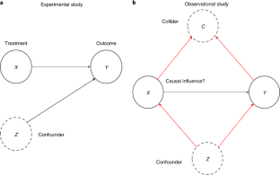
Stable learning establishes some common ground between causal inference and machine learning

Raiders of the lost HARK: a reproducible inference framework for big data science

Simple nested Bayesian hypothesis testing for meta-analysis, Cox, Poisson and logistic regression models
Code availability.
We provide interactive widgets of Figs. 2 – 4 in a Jupyter Notebook hosted in a public GitHub repository ( https://github.com/tliu526/causal-data-science-perspective ) and served through Binder (see link in the GitHub repository).
van Dyk, D. et al. ASA statement on the role of statistics in data science. Amstat News https://magazine.amstat.org/blog/2015/10/01/asa-statement-on-the-role-of-statistics-in-data-science/ (2015).
Pearl, J. The seven tools of causal inference, with reflections on machine learning. Commun. ACM 62 , 54–60 (2019).
Article Google Scholar
Hernán, M. A., Hsu, J. & Healy, B. Data science is science’s second chance to get causal inference right: a classification of data science tasks. Chance 32 , 42–49 (2019).
Caruana, R. et al. Intelligible models for healthcare: predicting pneumonia risk and hospital 30-day readmission. In Proc. 21th ACM SIGKDD International Conference on Knowledge Discovery and Data Mining 1721–1730 (ACM Press, 2015); https://doi.org/10.1145/2783258.2788613
Finkelstein, A. et al. The Oregon health insurance experiment: evidence from the first year. Q. J. Econ. 127 , 1057–1106 (2012).
Forney, A., Pearl, J. & Bareinboim, E. Counterfactual data-fusion for online reinforcement learners. In International Conference on Machine Learning (eds. Precup, D. & Teh, Y. W.) 1156–1164 (PMLR, 2017).
Thomas, P. S. & Brunskill, E. Data-efficient off-policy policy evaluation for reinforcement learning. International Conference on Machine Learning (eds. Balcan, M. F. & Weinberger, K.) 2139–2148 (PMLR, 2016).
Athey, S. & Wager, S. Policy learning with observational data. Econometrica (in the press).
Angrist, J. D. & Pischke, J.-S. Mostly Harmless Econometrics: An Empiricist’s Companion (Princeton Univ. Press, 2008).
Imbens, G. & Rubin, D. B. Causal Inference: For Statistics, Social and Biomedical Sciences: An Introduction (Cambridge Univ. Press 2015).
Pearl, J. Causality (Cambridge Univ. Press, 2009).
Hernán, M. A. & Robins, J. M. Causal Inference: What If (Chapman & Hall/CRC, 2020).
Pearl, J. Causal inference in statistics: an overview. Stat. Surv. 3 , 96–146 (2009).
Article MathSciNet MATH Google Scholar
Peters, J., Janzing, D. & Schölkopf, B. Elements of Causal Inference: Foundations and Learning Algorithms (MIT Press, 2017).
Rosenbaum, P. R. & Rubin, D. B. The central role of the propensity score in observational studies for causal effects. Biometrika 70 , 41–55 (1983).
Chernozhukov, V. et al. Double/debiased machine learning for treatment and structural parameters. Econ. J. 21 , C1–C68 (2018).
MathSciNet Google Scholar
Spirtes, P., Glymour, C. N. & Scheines, R. Causation, Prediction, and Search (MIT Press, 2000).
Schölkopf, B. Causality for machine learning. Preprint at https://arxiv.org/abs/1911.10500 (2019).
Mooij, J. M., Peters, J., Janzing, D., Zscheischler, J. & Schölkopf, B. Distinguishing cause from effect using observational data: methods and benchmarks. J. Mach. Learn. Res. 17 , 1103–1204 (2016).
MathSciNet MATH Google Scholar
Huang, B. et al. Causal discovery from heterogeneous/nonstationary data. J. Mach. Learn. Res. 21 , 1–53 (2020).
Wang, Y. & Blei, D. M. The blessings of multiple causes. J. Am. Stat. Assoc. 114 , 1574–1596 (2019).
Leamer, E. E. Let’s take the con out of econometrics. Am. Econ. Rev. 73 , 31–43 (1983).
Google Scholar
Angrist, J. D. & Pischke, J.-S. The credibility revolution in empirical economics: how better research design is taking the con out of econometrics. J. Econ. Perspect. 24 , 3–30 (2010).
Angrist, J. D. & Krueger, A. B. Instrumental variables and the search for identification: from supply and demand to natural experiments. J. Econ. Perspect. 15 , 69–85 (2001).
Angrist, J. D. & Krueger, A. B. Does compulsory school attendance affect schooling and earnings? Q. J. Econ. 106 , 979–1014 (1991).
Wooldridge, J. M. Econometric Analysis of Cross Section and Panel Data (MIT Press, 2010).
Angrist, J. D., Imbens, G. W. & Krueger, A. B. Jackknife instrumental variables estimation. J. Appl. Econom. 14 , 57–67 (1999).
Newhouse, J. P. & McClellan, M. Econometrics in outcomes research: the use of instrumental variables. Annu. Rev. Public Health 19 , 17–34 (1998).
Imbens, G. Potential Outcome and Directed Acyclic Graph Approaches to Causality: Relevance for Empirical Practice in Economics Working Paper No. 26104 (NBER, 2019); https://doi.org/10.3386/w26104
Hanandita, W. & Tampubolon, G. Does poverty reduce mental health? An instrumental variable analysis. Soc. Sci. Med. 113 , 59–67 (2014).
Angrist, J. D., Graddy, K. & Imbens, G. W. The interpretation of instrumental variables estimators in simultaneous equations models with an application to the demand for fish. Rev. Econ. Stud. 67 , 499–527 (2000).
Article MATH Google Scholar
Thistlethwaite, D. L. & Campbell, D. T. Regression-discontinuity analysis: an alternative to the ex post facto experiment. J. Educ. Psychol. 51 , 309–317 (1960).
Fine, M. J. et al. A prediction rule to identify low-risk patients with community-acquired pneumonia. N. Engl. J. Med. 336 , 243–250 (1997).
Lee, D. S. & Lemieux, T. Regression discontinuity designs in economics. J. Econ. Lit. 48 , 281–355 (2010).
Cattaneo, M. D., Idrobo, N. & Titiunik, R. A Practical Introduction to Regression Discontinuity Designs (Cambridge Univ. Press, 2019).
Imbens, G. & Kalyanaraman, K. Optimal Bandwidth Choice for the Regression Discontinuity Estimator Working Paper No. 14726 (NBER, 2009); https://doi.org/10.3386/w14726
Calonico, S., Cattaneo, M. D. & Titiunik, R. Robust data-driven inference in the regression-discontinuity design. Stata J. 14 , 909–946 (2014).
McCrary, J. Manipulation of the running variable in the regression discontinuity design: a density test. J. Econ. 142 , 698–714 (2008).
Imbens, G. & Lemieux, T. Regression discontinuity designs: a guide to practice. J. Economet. 142 , 615–635 (2008).
NCI funding policy for RPG awards. NIH: National Cancer Institute https://deainfo.nci.nih.gov/grantspolicies/finalfundltr.htm (2020).
NIAID paylines. NIH: National Institute of Allergy and Infectious Diseases http://www.niaid.nih.gov/grants-contracts/niaid-paylines (2020).
Keele, L. J. & Titiunik, R. Geographic boundaries as regression discontinuities. Polit. Anal. 23 , 127–155 (2015).
Card, D. & Krueger, A. B. Minimum Wages and Employment: A Case Study of the Fast Food Industry in New Jersey and Pennsylvania Working Paper No. 4509 (NBER, 1993); https://doi.org/10.3386/w4509
Ashenfelter, O. & Card, D. Using the Longitudinal Structure of Earnings to Estimate the Effect of Training Programs Working Paper No. 1489 (NBER, 1984); https://doi.org/10.3386/w1489
Angrist, J. D. & Krueger, A. B. in Handbook of Labor Economics Vol. 3 (eds. Ashenfelter, O. C. & Card, D.) 1277–1366 (Elsevier, 1999).
Athey, S. & Imbens, G. W. Identification and inference in nonlinear difference-in-differences models. Econometrica 74 , 431–497 (2006).
Abadie, A. Semiparametric difference-in-differences estimators. Rev. Econ. Stud. 72 , 1–19 (2005).
Lu, C., Nie, X. & Wager, S. Robust nonparametric difference-in-differences estimation. Preprint at https://arxiv.org/abs/1905.11622 (2019).
Besley, T. & Case, A. Unnatural experiments? estimating the incidence of endogenous policies. Econ. J. 110 , 672–694 (2000).
Nunn, N. & Qian, N. US food aid and civil conflict. Am. Econ. Rev. 104 , 1630–1666 (2014).
Christian, P. & Barrett, C. B. Revisiting the Effect of Food Aid on Conflict: A Methodological Caution (The World Bank, 2017); https://doi.org/10.1596/1813-9450-8171 .
Angrist, J. & Imbens, G. Identification and Estimation of Local Average Treatment Effects Technical Working Paper No. 118 (NBER, 1995); https://doi.org/10.3386/t0118
Hahn, J., Todd, P. & Van der Klaauw, W. Identification and estimation of treatment effects with a regression-discontinuity design. Econometrica 69 , 201–209 (2001).
Angrist, J. & Rokkanen, M. Wanna Get Away? RD Identification Away from the Cutoff Working Paper No. 18662 (NBER, 2012); https://doi.org/10.3386/w18662
Rothwell, P. M. External validity of randomised controlled trials: “To whom do the results of this trial apply?”. The Lancet 365 , 82–93 (2005).
Rubin, D. B. For objective causal inference, design trumps analysis. Ann. Appl. Stat. 2 , 808–840 (2008).
Chaney, A. J. B., Stewart, B. M. & Engelhardt, B. E. How algorithmic confounding in recommendation systems increases homogeneity and decreases utility. In Proc. 12th ACM Conference on Recommender Systems 224–232 (Association for Computing Machinery, 2018); https://doi.org/10.1145/3240323.3240370 .
Sharma, A., Hofman, J. M. & Watts, D. J. Estimating the causal impact of recommendation systems from observational data. In Proc. Sixteenth ACM Conference on Economics and Computation 453–470 (Association for Computing Machinery, 2015); https://doi.org/10.1145/2764468.2764488
Lawlor, D. A., Harbord, R. M., Sterne, J. A. C., Timpson, N. & Smith, G. D. Mendelian randomization: using genes as instruments for making causal inferences in epidemiology. Stat. Med. 27 , 1133–1163 (2008).
Article MathSciNet Google Scholar
Zhao, Q., Chen, Y., Wang, J. & Small, D. S. Powerful three-sample genome-wide design and robust statistical inference in summary-data Mendelian randomization. Int. J. Epidemiol. 48 , 1478–1492 (2019).
Moscoe, E., Bor, J. & Bärnighausen, T. Regression discontinuity designs are underutilized in medicine, epidemiology, and public health: a review of current and best practice. J. Clin. Epidemiol. 68 , 132–143 (2015).
Blake, T., Nosko, C. & Tadelis, S. Consumer heterogeneity and paid search effectiveness: a large-scale field experiment. Econometrica 83 , 155–174 (2015).
Dimick, J. B. & Ryan, A. M. Methods for evaluating changes in health care policy: the difference-in-differences approach. JAMA 312 , 2401–2402 (2014).
Kallus, N., Puli, A. M. & Shalit, U. Removing hidden confounding by experimental grounding. Adv. Neural Inf. Process. Syst. 31 , 10888–10897 (2018).
Zhang, J. & Bareinboim, E. Markov Decision Processes with Unobserved Confounders: A Causal Approach. Technical Report (R-23) (Columbia CausalAI Laboratory, 2016).
Mnih, V. et al. Human-level control through deep reinforcement learning. Nature 518 , 529–533 (2015).
Lansdell, B., Triantafillou, S. & Kording, K. Rarely-switching linear bandits: optimization of causal effects for the real world. Preprint at https://arxiv.org/abs/1905.13121 (2019).
Adadi, A. & Berrada, M. Peeking inside the black-box: a survey on explainable artificial intelligence (XAI). IEEE Access 6 , 52138–52160 (2018).
Zhao, Q. & Hastie, T. Causal interpretations of black-box models. J. Bus. Econ. Stat. 39 , 272–281 (2021).
Moraffah, R., Karami, M., Guo, R., Raglin, A. & Liu, H. Causal interpretability for machine learning—problems, methods and evaluation. ACM SIGKDD Explor. Newsl. 22 , 18–33 (2020).
Ribeiro, M. T., Singh, S. & Guestrin, C. ‘Why should I trust you?’: Explaining the predictions of any classifier. In Proc. 22nd ACM SIGKDD International Conference on Knowledge Discovery and Data Mining 1135–1144 (Association for Computing Machinery, 2016); https://doi.org/10.1145/2939672.2939778
Mothilal, R. K., Sharma, A. & Tan, C. Explaining machine learning classifiers through diverse counterfactual explanations. In Proc. 2020 Conference on Fairness, Accountability, and Transparency 607–617 (Association for Computing Machinery, 2020); https://doi.org/10.1145/3351095.3372850
Hooker, G. & Mentch, L. Please stop permuting features: an explanation and alternatives. Preprint at https://arxiv.org/abs/1905.03151 (2019).
Mullainathan, S. & Spiess, J. Machine learning: an applied econometric approach. J. Econ. Perspect. 31 , 87–106 (2017).
Belloni, A., Chen, D., Chernozhukov, V. & Hansen, C. Sparse models and methods for optimal instruments with an application to eminent domain. Econometrica 80 , 2369–2429 (2012).
Singh, R., Sahani, M. & Gretton, A. Kernel instrumental variable regression. Adv. Neural Inf. Process. Syst. 32 , 4593–4605 (2019).
Hartford, J., Lewis, G., Leyton-Brown, K. & Taddy, M. Deep IV: a flexible approach for counterfactual prediction. In Proc. 34th International Conference on Machine Learning Vol. 70 (eds. Precup, D. & Teh Y. W.) 1414–1423 (JMLR.org, 2017).
Athey, S., Bayati, M., Doudchenko, N., Imbens, G. & Khosravi, K. Matrix Completion Methods for Causal Panel Data Models Working Paper No. 25132 (NBER, 2018); https://doi.org/10.3386/w25132
Athey, S., Bayati, M., Imbens, G. & Qu, Z. Ensemble methods for causal effects in panel data settings. AEA Pap. Proc. 109 , 65–70 (2019).
Kennedy, E. H., Balakrishnan, S. & G’Sell, M. Sharp instruments for classifying compliers and generalizing causal effects. Ann. Stat. 48 , 2008–2030 (2020).
Kallus, N. Classifying treatment responders under causal effect monotonicity. In Proc. 36th International Conference on Machine Learning Vol. 97 (eds. Chaudhuri, K. & Salakhutdniov, R.) 3201–3210 (PMLR, 2019).
Li, A. & Pearl, J. Unit selection based on counterfactual logic. In Proc. Twenty-Eighth International Joint Conference on Artificial Intelligence (ed. Kraus, S.) 1793–1799 (International Joint Conferences on Artificial Intelligence Organization, 2019); https://doi.org/10.24963/ijcai.2019/248
Dong, Y. & Lewbel, A. Identifying the effect of changing the policy threshold in regression discontinuity models. Rev. Econ. Stat. 97 , 1081–1092 (2015).
Marinescu, I. E., Triantafillou, S. & Kording, K. Regression discontinuity threshold optimization. SSRN https://doi.org/10.2139/ssrn.3333334 (2019).
Varian, H. R. Big data: new tricks for econometrics. J. Econ. Perspect. 28 , 3–28 (2014).
Athey, S. & Imbens, G. W. Machine learning methods that economists should know about. Annu. Rev. Econ. 11 , 685–725 (2019).
Hudgens, M. G. & Halloran, M. E. Toward causal inference with interference. J. Am. Stat. Assoc. 103 , 832–842 (2008).
Graham, B. & de Paula, A. The Econometric Analysis of Network Data (Elsevier, 2019).
Varian, H. R. Causal inference in economics and marketing. Proc. Natl. Acad. Sci. USA 113 , 7310–7315 (2016).
Marinescu, I. E., Lawlor, P. N. & Kording, K. P. Quasi-experimental causality in neuroscience and behavioural research. Nat. Hum. Behav. 2 , 891–898 (2018).
Abadie, A. & Cattaneo, M. D. Econometric methods for program evaluation. Annu. Rev. Econ. 10 , 465–503 (2018).
Huang, A. & Levinson, D. The effects of daylight saving time on vehicle crashes in Minnesota. J. Safety Res. 41 , 513–520 (2010).
Lepperød, M. E., Stöber, T., Hafting, T., Fyhn, M. & Kording, K. P. Inferring causal connectivity from pairwise recordings and optogenetics. Preprint at bioRxiv https://doi.org/10.1101/463760 (2018).
Bor, J., Moscoe, E., Mutevedzi, P., Newell, M.-L. & Bärnighausen, T. Regression discontinuity designs in epidemiology. Epidemiol. Camb. Mass 25 , 729–737 (2014).
Chen, Y., Ebenstein, A., Greenstone, M. & Li, H. Evidence on the impact of sustained exposure to air pollution on life expectancy from China’s Huai River policy. Proc. Natl. Acad. Sci. USA 110 , 12936–12941 (2013).
Lansdell, B. J. & Kording, K. P. Spiking allows neurons to estimate their causal effect. Preprint at bioRxiv https://doi.org/10.1101/253351 (2019).
Patel, M. S. et al. Association of the 2011 ACGME resident duty hour reforms with mortality and readmissions among hospitalized medicare patients. JAMA 312 , 2364–2373 (2014).
Rishika, R., Kumar, A., Janakiraman, R. & Bezawada, R. The effect of customers’ social media participation on customer visit frequency and profitability: an empirical investigation. Inf. Syst. Res. 24 , 108–127 (2012).
Butsic, V., Lewis, D. J., Radeloff, V. C., Baumann, M. & Kuemmerle, T. Quasi-experimental methods enable stronger inferences from observational data in ecology. Basic Appl. Ecol. 19 , 1–10 (2017).
Download references
Acknowledgements
We thank R. Ladhania and B. Lansdell for their comments and suggestions on this work. We acknowledge support from National Institutes of Health grant R01-EB028162. T.L. is supported by National Institute of Mental Health grant R01-MH111610.
Author information
Authors and affiliations.
Department of Computer and Information Science, University of Pennsylvania, Philadelphia, PA, USA
Tony Liu & Lyle Ungar
Department of Bioengineering, University of Pennsylvania, Philadelphia, PA, USA
Konrad Kording
Department of Neuroscience, University of Pennsylvania, Philadelphia, PA, USA
You can also search for this author in PubMed Google Scholar
Contributions
T.L. helped write and prepare the manuscript. L.U. and K.K. jointly supervised this work and helped write the manuscript. All authors discussed the structure and direction of the manuscript throughout its development.
Corresponding author
Correspondence to Konrad Kording .
Ethics declarations
Competing interests.
The authors declare no competing interests.
Additional information
Peer review information Fernando Chirigati was the primary editor on this Perspective and managed its editorial process and peer review in collaboration with the rest of the editorial team. Nature Computational Science thanks Jesper Tegnér and the other, anonymous, reviewer(s) for their contribution to the peer review of this work.
Publisher’s note Springer Nature remains neutral with regard to jurisdictional claims in published maps and institutional affiliations.
Rights and permissions
Reprints and permissions
About this article
Cite this article.
Liu, T., Ungar, L. & Kording, K. Quantifying causality in data science with quasi-experiments. Nat Comput Sci 1 , 24–32 (2021). https://doi.org/10.1038/s43588-020-00005-8
Download citation
Received : 14 August 2020
Accepted : 30 November 2020
Published : 14 January 2021
Issue Date : January 2021
DOI : https://doi.org/10.1038/s43588-020-00005-8
Share this article
Anyone you share the following link with will be able to read this content:
Sorry, a shareable link is not currently available for this article.
Provided by the Springer Nature SharedIt content-sharing initiative
This article is cited by
Gendered beliefs about mathematics ability transmit across generations through children’s peers.
Nature Human Behaviour (2022)
Integrating explanation and prediction in computational social science
- Jake M. Hofman
- Duncan J. Watts
- Tal Yarkoni
Nature (2021)
Quick links
- Explore articles by subject
- Guide to authors
- Editorial policies
Sign up for the Nature Briefing: AI and Robotics newsletter — what matters in AI and robotics research, free to your inbox weekly.

- Open access
- Published: 13 September 2024
Test preparation breeds success: Two quasi-experimental interventions in the context of the Swiss aptitude test for medical-school admissions
- Petra L. Klumb 1 , 2 &
- Benjamin Spicher 2
BMC Medical Education volume 24 , Article number: 998 ( 2024 ) Cite this article
Metrics details
In Switzerland, the scholastic aptitude test for medical-school selection takes place in three languages. This study examined the effects of two quasi-experimental interventions that aimed to reduce existing differences in test results between the French- and German-speaking language candidates.
Between 2018 and 2023, the population of applicants to Swiss medical schools consisted of N = 18’824 German- and French-speaking individuals. Based on a quasi-experimental design, we examined the effects of two interventions regarding preparatory material, in these cohorts. The first intervention (2022) consisting of practice trials in baccalaureate schools in the canton of Fribourg enabled French-speaking candidates primarily from the canton of Fribourg to prepare more intensively with official tasks. Practice trials enable future candidates to complete a published test version under original conditions and thus prepare how to approach the real test. The second intervention (2023) released new preparatory material in all languages for one group of tasks for which differences between the language groups were more pronounced than in the other tasks. The test provider offered this material for free download together with existing preparation materials and thereby enabled more intensive preparation.
After the first intervention, the initially small to medium-sized mean differences in z-transformed test scores between French-speaking candidates from Fribourg and German-speaking candidates were nearly eliminated (from 0.39 to 0.05). Also for French-speaking candidates from outside of the canton of Fribourg, the mean differences were smaller than before the intervention (0.48 before, 0.39 after first intervention). After the second intervention, particularly the mean differences in test scores between German-speaking and French-speaking candidates from outside of Fribourg were further reduced (to 0.24).
Conclusions
The two interventions regarding material for preparing to participate in the aptitude test affected candidates’ test scores. They reduced the gap between German- and French-speaking candidates showing that the additional benefits of commercial offers for test preparation are limited. Hence, offering comparable official preparation material to all language groups enhances test fairness.
Peer Review reports
In many countries, standardized scholastic-aptitude test scores are employed in medical-school admissions to select candidates whose future academic performance will be high. Key criteria for the test procedures are predictive validity [ 1 , 2 , see also 3 , for a discussion of selection criteria], economy of administration, and – since most universities strive for diversity and inclusion – fairness. The procedural component of fairness encompasses consistency of administration across people and time [ 4 , 5 ]. An important aspect of this is ensuring access to information about the procedure and practice materials for all candidates. In multilingual countries such as Switzerland in which materials are provided in more than one language, this is particularly challenging.
Generally, existing research showed test-preparation information and activities such as practice trials to be positively related to applicant reactions [ 6 , 7 ] and, more importantly, to test performance (e.g., 8 – 10 , but see 11 , 12 , for studies that did not find effects probably due to shorter test preparation times). Most of this research relied on self-reported investment in preparation time, effort, or methods elicited either before [ 13 ] or after test administration [ 10 , 14 ]. As valuable as they are for examining effects of preparation, these studies have several limitations. First and foremost, survey participation or consent to linking survey response to outcomes may be related to participant characteristics. Secondly, when elicited after the test, the predictor “reported preparation information” may be contaminated by test experience or the outcome. Thirdly, participants may not be able to provide accurate judgments of their preparatory investment. Together, these limitations make it difficult to draw causal inferences and impair generalizability.
What is needed to complement existing observational research are investigations of all candidates who took a test within a specific period e.g., within a quasi-experimental approach. Quasi-experiments designate a group of non-randomized intervention studies typically with pre- and post-treatment measurements, in field settings [e.g., 15 , 16 ]. When random assignments are not possible, e.g., for ethical reasons, these approaches strengthen causal inferences by affording a higher degree of internal validity than observational designs. As a case in point, examining naturally occurring changes in access to practice materials allows researchers to avoid withholding this beneficial intervention from some candidates [ 16 ]. With our study, we aim to fill the described gap.
Setting and research question
In all German-speaking universities of Switzerland and in the bilingual University of Fribourg, access to medical school is restricted ( numerus clausus ). To be admitted to one of these universities, candidates from all over Switzerland have to pass the “aptitude test for medical studies” (EMS), in addition to having obtained a university-entrance qualification (“Maturität”). In each cohort, the proportion of individuals acquiring this entrance qualification varies substantially by canton (e.g., 33.6% for the canton of Geneva and 12.9% for the canton of Schaffhausen in 2021 [ 17 ]) and generally, this proportion is higher in French- as compared to German-speaking cantons.
Each year, the number of admitted applicants corresponds to the study places available. Depending on the exact number of applicants, roughly 35% of candidates for human medicine are admitted to the participating medical schools. Even small mean differences in test scores between groups can lead to substantial differences regarding the admission rate, due to different distributions, for instance.
The EMS is offered in three languages and its adaptation goes beyond translating the items. More important than merely capturing their original content is staying true to the intent and complexity of the text. Additionally, differential item functioning is analysed to identify and mitigate unwanted effects caused by the adaptation.
No matter from which canton a candidate originates, admission to the available places in the participating universities is granted solely according to the rank order of the test results. However, French-speaking persons can avoid the EMS by enrolling in one of the universities in Francophone cantons, where student numbers are not limited, in the first year. Therefore, French speakers taking the EMS are exclusively those who wish to begin their studies in Fribourg, or one of the German-speaking universities. Due to this self-selection among the French speakers as well as substantial differences in canton-specific education systems, identical results for the language groups are not necessarily to be expected.
Since many years, all participants have access to official information and preparation materials in all test languages via the webpage on which they register for the test. The official materials consist of three original test versions (formerly used test items), a test-information brochure explaining the administrative procedures for taking the test, as well as annotated sample exercises, approximately half the size of an original test. In addition, all Swiss baccalaureate schools are receiving relevant documents enabling them to implement practice trials, each year.
Importantly, there are commercial providers who sell unofficial preparation materials and courses. None of them contain original tasks. Because demand for German material is stronger than for material in other languages, these commercial materials and courses are only available in German. In contrast, the same official materials have been available since the first execution of the test in 1998, in all languages. Self-reports showed, however, that the use of official materials and particularly the time invested in test preparation differ between the language groups. In part, this may reflect the differential availability of commercial material across the languages.
For that reason, two interventions were carried out with the aim of making French-language offers primarily in the canton of Fribourg more comparable to school and other non-commercial offers in German-speaking cantons. This study examined whether the existing differences in test scores between German- and French-language groups would be reduced after two quasi-experimental interventions regarding access to preparation material for the EMS.
We investigated the effects of two quasi-experimental interventions regarding EMS preparation material on the total EMS score in three language groups (see below). The first intervention consisted of practice trials in baccalaureate schools in the canton of Fribourg, in 2022. Enabling French-speaking candidates primarily from the canton of Fribourg to prepare more intensively with official materials, the intervention was expected to result in higher levels of performance in the French-speaking group from Fribourg. The second intervention, in 2023, consisted in offering additional practice tasks of the type “concentrated and careful work”, in all test languages. Since differences between the language groups had been larger in this task group than in other tasks, we expected the intervention to benefit particularly French-speaking participants. A smaller effect of the intervention should arise in German-speaking participants for whom more commercial material was available - probably resulting in slowed growth in benefits. Hence, the gap that existed between German- and all French-speaking candidates should be reduced, after this intervention.
Participants
We included the complete population of 18’824 candidates who applied for a place in medical school and completed the test in German ( N = 17,690) or French ( N = 1134) between 2018 and 2023 (i.e., across 6 years). Those who took the test in French were further differentiated according to the canton of their school attendance (canton of Fribourg, N = 413 vs. other cantons, N = 721), as the measures offered by cantons were primarily introduced via the baccalaureate schools. Across the six years, 66.8% of the candidates were women, 33.2% were men. The mean age for almost all groups is higher for male participants as a substantial share of them usually complete their military service before applying to medical school. Table 1 displays the characteristics of the individual test cohorts.
Procedure and design
The aptitude tests were carried out at 32 test locations throughout Switzerland. German-speaking participants took part in one of the test locations in the German-speaking cantons. Based on their last name, French-speaking participants from Fribourg and from other cantons were assigned alphabetically to one of the two locations offering exclusively a French version of the test. The data represent the language-specific total population across the six years considered.
We employed a variant of an interrupted time-series design in which a string of equidistant independent observations was interrupted by two interventions taking place in 2022 and 2023. Prior to the 2022 test administration, Intervention 1 was introduced enabling future French-speaking participants - primarily from the canton of Fribourg - to prepare more intensively with official materials. The intervention that was officially supported by the Department of Education and Cultural Affairs of the canton of Fribourg consisted in coordinated practice trials with original tasks of all task types, mainly offered by baccalaureate schools, outside of teaching time. In addition, practice tasks were developed on an honorary basis and made available online by a group of medical students, who also organized trial runs in the rooms of the University of Fribourg. To the best of our knowledge, there was no increase in the availability of commercial materials in French, during this period.
Prior to the 2023 test administration, Intervention 2 was introduced by the test provider. It consisted in the provision of additional original tasks of the type “concentrated and careful work”, in all test languages. For this purpose, former tasks were made available for free download, together with corresponding norm tables enabling direct comparisons with the empirical test data. The use of these materials for preparation was hence independent of participants’ place of residence.
Language group
Categorized according to their language and place of residence, there were three groups of participants. These were German-speaking participants (g), French-speaking participants from Fribourg (f fr ) as well as French-speaking participants from other cantons (f o ).
Year of test participation (test cohort)
In the years from 2018 until 2021 (t 0 ), there were no interventions. As described above, in 2022 (t 1 ), Intervention 1 was implemented focusing on the canton of Fribourg. In 2023 (t 2 ), Intervention 2 was available for all potential candidates.
Outcome: total EMS score
We used the year-specific z-transformed total scores of the aptitude test for medical studies as dependent variable that is comparable across the six years.
Data analyses
Employing the Statistical Package for the Social Sciences Version 29, we standardized aptitude test scores via z-transformations and computed mean z-scores as well as Cohen’s d with a local type-I-error level of alpha = 0.05.
Descriptive information
Table 2 depicts z-values for the groups across the six years. Before the first intervention in 2022, the German-speaking group achieved z-scores of approximately 0.02 to 0.03. In 2022, the score decreased to less than 0.02, and in 2023 it decreased further to 0.01. At the same time, the z-scores for the French-speaking group from outside of the canton of Fribourg decreased in absolute terms from − 0.40 to − 0.37 after the first intervention, and then to − 0.23 after the second intervention. The difference for the Fribourg-based French-speaking group was smaller to begin with (z-score of − 0.37 just before the first intervention). After the first intervention, the remaining difference was very small (z-score of − 0.03) and decreased further after the second intervention (-0.02).
Effect of the interventions
After both interventions, there were still differences between the three participant groups. As expected, the initially small to medium-sized effects (Cohen’s d, see Fig. 1 ) were reduced after both interventions to very small remaining differences in the French speakers from Fribourg and to still medium-sized effects that were smaller than before the interventions for those from other cantons. As expected, Intervention 1 primarily affected French-speaking participants from the canton of Fribourg (ffr). The mean difference between these and German-speaking candidates decreased from 0.39 to 0.05, no longer differing beyond unsystematic variation. The mean difference between French speakers from other cantons (fo) and German speakers shrank from 0.48 to 0.39, during this period. After Intervention 2, scores of both French-speaking groups further converged with those of the German-speaking group. The mean differences were 0.24 for fo, and 0.03 for ffr.

Cohen’s d for differences between French speaking groups and German-speaking group (with 95% confidence interval and a local type-I-error level of alpha = 0.05, exact numbers are provided in supplementary material, Table 1 ). Notes. ffr: French-speaking participants from canton Fribourg, fo: participants from French-speaking cantons other than Fribourg
Before the first measure, the German-speaking groups differed from both French-speaking groups, which did not differ from each other. The first intervention led to an improvement in both French-speaking groups, with candidates from schools in the canton of Fribourg benefitting more than other French speakers. There were no longer reliable differences between the French-speaking group from Fribourg and the German-speaking group, but there still was an observable difference between the two French-speaking groups. After the second intervention, the difference between German-speaking participants and those who attended school outside of Fribourg was further reduced. There were no longer reliable differences between the two French-speaking groups.
Based on two quasi-experimental interventions, we investigated the effects of the availability of test preparation materials on test performance. The intervention that focused on candidates from the canton Fribourg differentially affected test scores, in this group. The intervention for all language groups benefitted both French-speaking groups more than the German-speaking group. We expected these diminishing marginal returns in the latter group since non-official, commercial material was already widely available in German. After the two interventions, the preexisting differences between the two language groups were no longer present. Our findings confirm the beneficial effects of test preparation reported by previous studies that primarily assessed preparatory activities via self-report (e.g., 7 – 9 ).
The quasi-experimental approach allowed us to attribute changes in test scores to the two introduced changes in the availability of free practice material. Several potential alternative explanations of the reported effects can be excluded. First of all, the process of adapting items from German into French did not change during the period included. Potential translation-related effects thus cannot explain the effects. Also, to the best of our knowledge, no additional commercial preparation offers in French were made available. Moreover, while children of parents with higher education are more likely to obtain a university entrance qualification and parents’ income may play role for access to commercial preparation material, neither economic nor social or cultural resources are relevant regarding access to official preparation material. The latter is available for free via baccalaureate schools and via the webpage where candidates register for the test. Finally, an effect based on changed compositions of the participants seems unlikely due to the relative stability of the differences before 2022.
Since the whole population was investigated there is no generalizability issue within Switzerland. It should also be possible to generalize our findings to similar multilingual countries such as Belgium or Canada since they share Switzerland’s linguistic diversity and decentralized education systems making them similar in socio-cultural respect. Our findings may not be directly transferable to India, Israel, or South Africa, however, because of their complex socio-cultural, political, and historical contexts and their higher linguistic diversity.
Transfer to other selection settings such as personnel selection (e.g., 7 ) or admission to highly selective colleges [e.g., 3 ] is possible since key features of the selection processes are comparable to those in medical-school admission. Generally, facilitating access to consistent information about test content and procedures allows all participants to realize their potential and participants with the same ability level can expect to achieve the same test result – regardless of their language or other characteristics. This is a core feature of fair selection processes. By providing comparable opportunities for preparation, institutions can reduce factors that systematically bias inferences regarding performance criteria (i.e., future grades) thereby enhancing the predictive validity of the applied procedure. As a consequence, test motivation of candidates was shown to be higher and the number of appeals lower [e.g., 4 ].
Strengths and limitations
All candidates who took part in the test between 2018 and 2023 were included in the study. Hence, this study minimized validity threats to causality although participants were not randomly assigned to treatment conditions. While the small to medium-sized differences between the language groups have shown to be relatively stable over the years (see Fig. 1 ), we acknowledge that there were only two data points after the first intervention. In future EMS cohorts, we would expect some variance to remain between the language groups, but it should be smaller than before the interventions. Finally, since we do not possess information regarding socio-economic status, we could not determine the probable influence of this factor on test performance. Since it is not likely that large changes in the composition of language groups occurred in the observation period, the reported intervention effects are unlikely to be a function of socio-economic differences between these groups.
Our findings show a clear pattern of test results in the three language groups converging after the interventions. These effects underline the importance of making comparable preparation material freely available to all candidates. While standardized test scores as admissions criterion already provide broader access than alternative procedures such as non-academic ratings [ 3 ], test fairness is further enhanced by this intervention. At the same time, additional benefits of commercial offers for the preparation of scholastic aptitude tests are apparently limited.
Data availability
Data of this study are deposited in SWISSUbase under the reference 20717.
Hell B, Trappmann. Sabrina, Schuler, Heinz. Eine Metaanalyse Der Validität Von Fachspezifischen Studierfähigkeitstests Im Deutschsprachigen Raum. [A meta-analysis of the validity of subject-specific scholastic aptitude tests in german-speaking regions]. Empirische Pädagogik. 2007;21(3):251–70.
Google Scholar
Kuncel NR, Credé M, Thomas LL. The validity of self-reported Grade Point averages, Class Ranks, and test scores: a Meta-analysis and review of the literature. Rev Educ Res. 2005;75(1):63–82.
Article Google Scholar
Chetty R, Deming DJ, Friedman JN. Diversifying society’s leaders? The determinants and causal effects of admission to highly selective private colleges. NBER working paper 31492. http://www.nber.org/papers/w31492
Gilliland SW, Steiner DD. Applicant Reactions to Testing and Selection. In: Schmitt N, editor. The Oxford Handbook of Personnel Assessment and Selection [Internet]. 1st ed. Oxford University Press; 2012 [cited 2024 Mar 8]. pp. 629–66. https://academic.oup.com/edited-volume/28202/chapter/213200238
Tippins NT, Sackett PR. Oswald, Fred. Principles for the Validation and Use of Personnel Selection procedures | Fifth Edition. 5th ed. Bowling Green, OH: Society Industrial Organizational Psychology.
Denker M, Schütte C, Kersting M, Weppert D, Stegt SJ. How can applicants’ reactions to scholastic aptitude tests be improved? A closer look at specific and general tests. Front Educ. 2023;7:931841.
Lievens F, De Corte W, Brysse K. Applicant perceptions of selection procedures: the role of selection information, belief in tests, and comparative anxiety. Int J Sel Assess. 2003;11(1):67–77.
Clause CS, Delbridge K, Schmitt N, Chan D, Jennings D. Test Preparation activities and Employment Test performance. Hum Perform. 2001;14(2):149–67.
Jackson D, Ward D, Agwu JC, Spruce A. Preparing for selection success: Socio-demographic differences in opportunities and obstacles. Med Educ. 2022;56(9):922–35.
Laurence CO, Zajac IT, Lorimer M, Turnbull DA, Sumner KE. The impact of preparatory activities on medical school selection outcomes: a cross-sectional survey of applicants to the university of Adelaide medical school in 2007. BMC Med Educ. 2013;13(1):159–68.
Burns GN, Siers BP, Christiansen ND. Effects of providing Pre-test Information and Preparation materials on applicant reactions to selection procedures. Int J Sel Assess. 2008;16(1):73–7.
Ryan AM, Ployhart RE, Greguras GJ, Schmit MJ. Test preparation programs in selection contexts: self-selection and program effectiveness. Pers Psychol. 1998;51(3):599–621.
Weppert D, Amelung D, Escher M, Troll L, Kadmon M, Listunova L et al. The impact of preparatory activities on the largest clinical aptitude test for prospective medical students in Germany. Front Educ [Internet]. 2023 [cited 2024 Feb 15];8. https://www.frontiersin.org/articles/ https://doi.org/10.3389/feduc.2023.1104464
Kulkarni S, Parry J, Sitch A. An assessment of the impact of formal preparation activities on performance in the University Clinical Aptitude Test (UCAT): a national study. BMC Med Educ. 2022;22(1):747–60.
Harris AD, McGregor JC, Perencevich EN, Furuno JP, Zhu J, Peterson DE, et al. The Use and Interpretation of Quasi-experimental studies in Medical Informatics. J Am Med Inf Assoc. 2006;13(1):16–23.
Grant AM, Wall TD. The Neglected Science and Art of Quasi-experimentation: Why-to, When-to, and how-to advice for Organizational Researchers. Organ Res Methods. 2009;12(4):653–86.
Bundesamt für Statistik. Längschnittanalysen im Bildungsbereich [Longitudinal analyses in the education sector]; https://www.bfs.admin.ch/asset/de/28905348 . Accessed 31 July 2024.
Download references
Not Applicable.
Author information
Authors and affiliations.
Department of Psychology and Center for Test Development and Diagnostics, University of Fribourg, rue de Faucigny 2, Fribourg, 1700, Switzerland
Petra L. Klumb
Center for Test Development and Diagnostics, University of Fribourg, Fribourg, Switzerland
Petra L. Klumb & Benjamin Spicher
You can also search for this author in PubMed Google Scholar
Contributions
plk conceptualized and wrote the original draft, B.Sp. curated and analyzed the data, and prepared Fig. 1, B.Sp. and plk took methodological decisions and reviewed and edited the draft.
Corresponding author
Correspondence to Petra L. Klumb .
Ethics declarations
Ethics approval and consent to participate.
The local Ethics Committee waived the need for approval (29 FEB 2024).
Consent for publication
Competing interests.
Petra Klumb is director of the Center for Test Development and Diagnostics and Benjamin Spicher is scientific collaborator at the Center for Test Development and Diagnostics, University of Fribourg, where the scholastic aptitude test EMS is developed, translated, and administered.
Additional information
Publisher’s note.
Springer Nature remains neutral with regard to jurisdictional claims in published maps and institutional affiliations.
Electronic supplementary material
Below is the link to the electronic supplementary material.
Supplementary Material 1
Rights and permissions.
Open Access This article is licensed under a Creative Commons Attribution-NonCommercial-NoDerivatives 4.0 International License, which permits any non-commercial use, sharing, distribution and reproduction in any medium or format, as long as you give appropriate credit to the original author(s) and the source, provide a link to the Creative Commons licence, and indicate if you modified the licensed material. You do not have permission under this licence to share adapted material derived from this article or parts of it. The images or other third party material in this article are included in the article’s Creative Commons licence, unless indicated otherwise in a credit line to the material. If material is not included in the article’s Creative Commons licence and your intended use is not permitted by statutory regulation or exceeds the permitted use, you will need to obtain permission directly from the copyright holder. To view a copy of this licence, visit http://creativecommons.org/licenses/by-nc-nd/4.0/ .
Reprints and permissions
About this article
Cite this article.
Klumb, P.L., Spicher, B. Test preparation breeds success: Two quasi-experimental interventions in the context of the Swiss aptitude test for medical-school admissions. BMC Med Educ 24 , 998 (2024). https://doi.org/10.1186/s12909-024-05971-5
Download citation
Received : 21 March 2024
Accepted : 29 August 2024
Published : 13 September 2024
DOI : https://doi.org/10.1186/s12909-024-05971-5
Share this article
Anyone you share the following link with will be able to read this content:
Sorry, a shareable link is not currently available for this article.
Provided by the Springer Nature SharedIt content-sharing initiative
- Medical-school admissions
- Student selection procedures
- Scholastic aptitude test
- Test preparation information
- Practice materials
BMC Medical Education
ISSN: 1472-6920
- General enquiries: [email protected]
An official website of the United States government
The .gov means it’s official. Federal government websites often end in .gov or .mil. Before sharing sensitive information, make sure you’re on a federal government site.
The site is secure. The https:// ensures that you are connecting to the official website and that any information you provide is encrypted and transmitted securely.
- Publications
- Account settings
Preview improvements coming to the PMC website in October 2024. Learn More or Try it out now .
- Advanced Search
- Journal List
- HHS Author Manuscripts
Quasi-Experimental Designs for Causal Inference
When randomized experiments are infeasible, quasi-experimental designs can be exploited to evaluate causal treatment effects. The strongest quasi-experimental designs for causal inference are regression discontinuity designs, instrumental variable designs, matching and propensity score designs, and comparative interrupted time series designs. This article introduces for each design the basic rationale, discusses the assumptions required for identifying a causal effect, outlines methods for estimating the effect, and highlights potential validity threats and strategies for dealing with them. Causal estimands and identification results are formalized with the potential outcomes notations of the Rubin causal model.
Causal inference plays a central role in many social and behavioral sciences, including psychology and education. But drawing valid causal conclusions is challenging because they are warranted only if the study design meets a set of strong and frequently untestable assumptions. Thus, studies aiming at causal inference should employ designs and design elements that are able to rule out most plausible threats to validity. Randomized controlled trials (RCTs) are considered as the gold standard for causal inference because they rely on the fewest and weakest assumptions. But under certain conditions quasi-experimental designs that lack random assignment can also be as credible as RCTs ( Shadish, Cook, & Campbell, 2002 ).
This article discusses four of the strongest quasi-experimental designs for identifying causal effects: regression discontinuity design, instrumental variable design, matching and propensity score designs, and the comparative interrupted time series design. For each design we outline the strategy and assumptions for identifying a causal effect, address estimation methods, and discuss practical issues and suggestions for strengthening the basic designs. To highlight the design differences, throughout the article we use a hypothetical example with the following causal research question: What is the effect of attending a summer science camp on students’ science achievement?
POTENTIAL OUTCOMES AND RANDOMIZED CONTROLLED TRIAL
Before we discuss the four quasi-experimental designs, we introduce the potential outcomes notation of the Rubin causal model (RCM) and show how it is used in the context of an RCT. The RCM ( Holland, 1986 ) formalizes causal inference in terms of potential outcomes, which allow us to precisely define causal quantities of interest and to explicate the assumptions required for identifying them. RCM considers a potential outcome for each possible treatment condition. For a dichotomous treatment variable (i.e., a treatment and control condition), each subject i has a potential treatment outcome Y i (1), which we would observe if subject i receives the treatment ( Z i = 1), and a potential control outcome Y i (0), which we would observe if subject i receives the control condition ( Z i = 0). The difference in the two potential outcomes, Y i (1)− Y i (0), represents the individual causal effect.
Suppose we want to evaluate the effect of attending a summer science camp on students’ science achievement score. Then each student has two potential outcomes: a potential control score for not attending the science camp, and the potential treatment score for attending the camp. However, the individual causal effects of attending the camp cannot be inferred from data, because the two potential outcomes are never observed simultaneously. Instead, researchers typically focus on average causal effects. The average treatment effect (ATE) for the entire study population is defined as the difference in the expected potential outcomes, ATE = E [ Y i (1)] − E [ Y i (0)]. Similarly, we can also define the ATE for the treated subjects (ATT), ATT = E [ Y i (1) | Z i = 1] − E [ Y (0) | Z i =1]. Although the expectations of the potential outcomes are not directly observable because not all potential outcomes are observed, we nonetheless can identify ATE or ATT under some reasonable assumptions. In an RCT, random assignment establishes independence between the potential outcomes and the treatment status, which allows us to infer ATE. Suppose that students are randomly assigned to the science camp and that all students comply with the assigned condition. Then random assignment guarantees that the camp attendance indicator Z is independent of the potential achievement scores Y i (0) and Y i (1).
The independence assumption allows us to rewrite ATE in terms of observable expectations (i.e., with observed outcomes instead of potential outcomes). First, due to the independence (randomization), the unconditional expectations of the potential outcomes can be expressed as conditional expectations, E [ Y i (1)] = E [ Y i (1) | Z i = 1] and E [ Y i (0)] = E [ Y i (0) | Z i = 0] Second, because the potential treatment outcomes are actually observed for the treated, we can replace the potential treatment outcome with the observed outcome such that E [ Y i (1) | Z i = 1] = E [ Y i | Z i = 1] and, analogously, E [ Y i (0) | Z i = 0] = E [ Y i | Z i = 0] Thus, the ATE is expressible in terms of observable quantities rather than potential outcomes, ATE = E [ Y i (1)] − E [ Y i (0)] = E [ Y i | Z i = 1] – E [ Y i | Z i = 0], and we that say ATE is identified.
This derivation also rests on the stable-unit-treatment-value assumption (SUTVA; Imbens & Rubin, 2015 ). SUTVA is required to properly define the potential outcomes, that is, (a) the potential outcomes of a subject depend neither on the assignment mode nor on other subjects’ treatment assignment, and (b) there is only one unique treatment and one unique control condition. Without further mentioning, we assume SUTVA for all quasi-experimental designs discussed in this article.
REGRESSION DISCONTINUITY DESIGN
Due to ethical or budgetary reasons, random assignment is often infeasible in practice. Nonetheless, researchers may sometimes still retain full control over treatment assignment as in a regression discontinuity (RD) design where, based on a continuous assignment variable and a cutoff score, subjects are deterministically assigned to treatment conditions.
Suppose that the science camp is a remedial program and only students whose grade point average (GPA) score is less than or equal to 2.0 are eligible to participate. Figure 1 shows a scatterplot of hypothetical data where the x-axis represents the assignment variable ( GPA ) and the y -axis the outcome ( Science Score ). All subjects with a GPA score below the cutoff attended the camp (circles), whereas all subjects scoring above the cutoff do not attend (squares). Because all low-achieving students are in the treatment group and all high-achieving students in the control group, their respective GPA distributions do not overlap, not even at the cutoff. This lack of overlap complicates the identification of a causal effect because students in the treatment and control group are not comparable at all (i.e., they have a completely different distribution of the GPA scores).

A hypothetical example of regression discontinuity design. Note . GPA = grade point average.
One strategy of dealing with the lack of overlap is to rely on the linearity assumption of regression models and to extrapolate into areas of nonoverlap. However, if the linear models do not correctly specify the functional form, the resulting ATE estimate is biased. A safer strategy is to evaluate the treatment effect only at the cutoff score where treatment and control cases almost overlap, and thus functional form assumptions and extrapolation are almost no longer needed. Consider the treatment and control students that score right at the cutoff or just above it. Students with a GPA score of 2.0 participate in the science camp and students with a GPA score of 2.1 are in the control condition (the status quo condition or a different camp). The two groups of students are essentially equivalent because the difference in their GPA scores is negligibly small (2.1 − 2.0 = .1) and likely due to random chance (measurement error) rather than a real difference in ability. Thus, in the very close neighborhood around the cutoff score, the RD design is equivalent to an RCT; therefore, the ATE at the cutoff (ATEC) is identified.
CAUSAL ESTIMAND AND IDENTIFICATION
ATEC is defined as the difference in the expected potential treatment and control outcomes for the subjects scoring exactly at the cutoff: ATEC = E [ Y i (1) | A i = a c ] − E [ Y i (0) | A i = a c ], where A denotes assignment variable and a c the cutoff score. Because we observe only treatment subjects and not control subjects right at the cutoff, we need two assumptions in order to identify ATEC ( Hahn, Todd, & van Klaauw, 2001 ): (a) the conditional expectations of the potential treatment and control outcomes are continuous at the cutoff ( continuity ), and (b) all subjects comply with treatment assignment ( full compliance ).
The continuity assumption can be expressed in terms of limits as lim a ↓ a C E [ Y i ( 1 ) | A i = a ] = E [ Y i ( 1 ) | A i = a ] = lim a ↑ a C E [ Y i ( 1 ) | A i = a ] and lim a ↓ a C E [ Y i ( 0 ) | A i = a ] = E [ Y i ( 0 ) | A i = a ] = lim a ↑ a C E [ Y i ( 0 ) | A i = a ] . Thus, we can rewrite ATEC as the difference in limits, A T E C = lim a ↑ a C E [ Y i ( 1 ) | A i = a c ] − lim a ↓ a C E [ Y i ( 0 ) | A i = a c ] , which solves the issue that no control subjects are observed directly at the cutoff. Then, by the full compliance assumption, the potential treatment and control outcomes can be replaced with the observed outcomes such that A T E C = lim a ↑ a C E [ Y i | A i = a c ] − lim a ↓ a C E [ Y i | A i = a c ] is identified at the cutoff (i.e., ATEC is now expressed in terms of observable quantities). The difference in the limits represents the discontinuity in the mean outcomes exactly at the cutoff ( Figure 1 ).
Estimating ATEC
ATEC can be estimated with parametric or nonparametric regression methods. First, consider the parametric regression of the outcome Y on the treatment Z , the cutoff-centered assignment variable A − a c , and their interaction: Y = β 0 + β 1 Z + β 2 ( A − a c ) + β 3 ( Z × ( A − a c )) + e . If the model correctly specifies the functional form, then β ^ 1 is an unbiased estimator for ATEC. In practice, an appropriate model specification frequently involves also quadratic and cubic terms of the assignment variable plus their interactions with the treatment indicator.
To avoid overly strong functional form assumptions, semiparametric or nonparametric regression methods like generalized additive models or local linear kernel regression can be employed ( Imbens & Lemieux, 2008 ). These methods down-weight or even discard observations that are not in the close neighborhood around the cutoff. The R packages rdd ( Dimmery, 2013 ) and rdrobust ( Calonico, Cattaneo, & Titiunik, 2015 ), or the command rd in STATA ( Nichols, 2007 ) are useful for estimation and diagnostic purposes.
Practical Issues
A major validity threat for RD designs is the manipulation of the assignment score around the cutoff, which directly results in a violation of the continuity assumption ( Wong et al., 2012 ). For instance, if a teacher knows the assignment score in advance and he wants all his students to attend the science camp, the teacher could falsely report a GPA score of 2.0 or below for the students whose actual GPA score exceeds the cutoff value.
Another validity threat is noncompliance, meaning that subjects assigned to the control condition may cross over to the treatment and subjects assigned to the treatment do not show up. An RD design with noncompliance is called a fuzzy RD design (instead of a sharp RD design with full compliance). A fuzzy RD design still allows us to identify the intention-to-treat effect or the local average treatment effect at the cutoff (LATEC). The intention-to-treat effect refers to the effect of treatment assignment rather than the actual treatment receipt. LATEC estimates ATEC for the subjects who comply with treatment assignment. LATEC is identified if one uses the assignment status as an instrumental variable for treatment receipt (see the upcoming Instrumental Variable section).
Finally, generalizability and statistical power are often mentioned as major disadvantages of RD designs. Because RD designs identify the treatment effect only at the cutoff, ATEC estimates are not automatically generalizable to subjects scoring further away from the cutoff. Statistical power for detecting a significant effect is an issue because the lack of overlap on the assignment variable results in increased standard errors. With semi- or nonparametric regression methods, power further diminishes.
Strengthening RD Designs
To avoid systematic manipulations of the assignment variable, it is desirable to conceal the assignment rule from study participants and administrators. If the assignment rule is known to them, manipulations can hardly be ruled out, particularly when the stakes are high. Researchers can use the McCrary test ( McCrary, 2008 ) to check for potential manipulations. The test investigates whether there is a discontinuity in the distribution of the assignment variable right at the cutoff. Plotting baseline covariates against the assignment variable, and regressing the covariates on the assignment variable and the treatment indicator also help in detecting potential discontinuities at the cutoff.
The RD design’s validity can be increased by combining the basic RD design with other designs. An example is the tie-breaking RD design, which uses two cutoff scores. Subjects scoring between the two cutoff scores are randomly assigned to treatment conditions, whereas subjects scoring outside the cutoff interval receive the treatment or control condition according to the RD assignment rule ( Black, Galdo & Smith, 2007 ). This design combines an RD design with an RCT and is advantageous with respect to the correct specification of the functional form, generalizability, and statistical power. Similar benefits can be obtained by adding pretest measures of the outcome or nonequivalent comparison groups ( Wing & Cook, 2013 ).
Imbens and Lemieux (2008) and Lee and Lemieux (2010) provided comprehensive introductions to RD designs. Lee and Lemieux also summarized many applications from economics. Angrist and Lavy (1999) applied the design to investigate the effect of class size on student achievement.
INSTRUMENTAL VARIABLE DESIGN
In practice, researchers often have no or only partial control over treatment selection. In addition, they might also lack reliable knowledge of the selection process. Nonetheless, even with limited control and knowledge of the selection process it is still possible to identify a causal treatment effect if an instrumental variable (IV) is available. An IV is an exogenous variable that is related to the treatment but is completely unrelated to the outcome, except via treatment. An IV design requires researchers either to create an IV at the design stage (as in an encouragement design; see next) or to find an IV in the data set at hand or a related data base.
Consider the science camp example, but instead of random or deterministic treatment assignment, students decide on their own or together with their parents whether to attend the camp. Many factors may determine the decision, for instance, students’ science ability and motivation, parents’ socioeconomic status, or the availability of public transportation for the daily commute to the camp. Whereas the first three variables are presumably also related to the science outcome, public transportation might be unrelated to the science score (except via camp attendance). Thus, the availability of public transportation may qualify as an IV. Figure 2 illustrates such IV design: Public transportation (IV) directly affects camp attendance but has no direct or indirect effect on science achievement (outcome) other than through camp attendance (treatment). The question mark represents unknown or unobserved confounders, that is, variables that simultaneously affect both camp attendance and science achievement. The IV design allows us to identify a causal effect even if some or all confounders are unknown or unobserved.

A diagram of an example of instrumental variable design.
The strategy for identifying a causal effect is based on exploiting the variation in the treatment variable explained by IV. In Figure 2 , the total variation in the treatment consists of (a) the variation induced by the IV and (b) the variation induced by confounders (question mark) and other exogenous variables (not shown in the figure). The identification of the camp’s effect requires us to isolate the treatment variation that is related to public transportation (IV), and then to use the isolated variation to investigate the camp’s effect on the science score. Because we exploit the treatment variation exclusively induced by the IV but ignore the variation induced by unobserved or unknown confounders, the IV design identifies the ATE for the sub-population of compliers only. In our example, the compliers are the students who attend the camp because public transportation is available and do not attend because it is unavailable. For students whose parents always use their own car to drop them off and pick them up at the camp location, we cannot infer the causal effect, because their camp attendance is completely unrelated to the availability of public transportation.
Causal Estimand and Identification
The complier average treatment effect (CATE) is defined as the expected difference in potential outcomes for the sub-population of compliers: CATE = E [ Y i (1) | Complier ] − E [ Y i (0) | Complier ] = τ C .
Identification requires us to distinguish between four latent groups: compliers (C), who attend the camp if public transportation is available but do not attend if unavailable; always-takers (A), who always attend the camp regardless of whether or not public transportation is available; never-takers (N), who never attend the camp regardless of public transportation; and defiers (D), who do not attend if public transportation is available but attend if unavailable. Because group membership is unknown, it is impossible to directly infer CATE from the data of compliers. However, CATE is identified from the entire data set if (a) the IV is predictive of the treatment ( predictive first stage ), (b) the IV is unrelated to the outcome except via treatment ( exclusion restriction ), and (c) no defiers are present ( monotonicity ; Angrist, Imbens, & Rubin, 1996 ; see Steiner, Kim, Hall, & Su, 2015 , for a graphical explanation).
First, notice that the IV’s effects on the treatment (γ) and the outcome (δ) are directly identified from the observed data because the IV’s relation with the treatment and outcome is unconfounded. In our example ( Figure 2 ), γ denotes the effect of public transportation on camp attendance and δ the indirect effect of public transportation on the science score. Both effects can be written as weighted averages of the corresponding group-specific effects ( γ C , γ A , γ N , γ D and δ C , δ A , δ N , δ D for compliers, always-takers, never-takers, and defiers, respectively): γ = p ( C ) γ C + p ( A ) γA + p ( N ) γ N + p ( D ) γ D and δ = p ( C ) δ C + p ( A ) δ A + p ( N ) δ N + p ( D ) δ D where p (.) represents the portion of the respective latent group in the population and p ( C ) + p ( A ) + p ( N ) + p ( D ) = 1. Because the treatment choice of always-takers and never-takers is entirely unaffected by the instrument, the IV’s effect on the treatment is zero, γ A = γ N = .0, and together with the exclusion restriction , we also know δ A = δ N = 0, that is, the IV has no effect on the outcome. If no defiers are present, p ( D ) = 0 ( monotonicity ), then the IV’s effects on the treatment and outcome simplify to γ = p ( C ) γC and δ = p ( C ) δC , respectively. Because δ C = γ C τ C and γ ≠ 0 ( predictive first stage ), the ratio of the observable IV effects, γ and δ, identifies CATE: δ γ = p ( C ) γ C τ C p ( C ) γ C = τ C .
Estimating CATE
A two-stage least squares (2SLS) regression is typically used for estimating CATE. In the first stage, treatment Z is regressed on the IV, Z = β 0 + β 1 IV + e . The linear first-stage model applies with a dichotomous treatment variable (linear probability model). The second stage then regresses the outcome Y on the predicted values Z ^ from the first stage model, Y = π 0 + π 1 Z ^ + r , where π ^ 1 is the CATE estimator. The two stages are automatically performed by the 2SLS procedure, which also provides an appropriate standard error for the effect estimate. The STATA commands ivregress and ivreg2 ( Baum, Schaffer, & Stillman, 2007 ) or the sem package in R ( Fox, 2006 ) perform the 2SLS regression.
One challenge in implementing an IV design is to find a valid instrument that satisfies the assumptions just discussed. In particular, the exclusion restriction is untestable and frequently hard to defend in practice. In our example, if high-income families live in suburban areas with bad public transportation connections, then the availability of the public transportation is likely related to the science score via household income (or socioeconomic status). Although conditioning on the observed household income can transform public transportation into a conditional IV (see next), one can frequently come up with additional scenarios that explains why the IV is related to the outcome and thus violates the exclusion restriction.
Another issue arises from “weak” IVs that are only weakly related to treatment. Weak IVs cause efficiency problems ( Wooldridge, 2012 ). If the availability of public transportation barely affects camp attendance because most parents give their children a ride anyway, the IV’s effect on the treatment ( γ ) is close to zero. Because γ ^ is the denominator in the CATE estimator, τ ^ C = δ ^ / γ ^ , an imprecisely estimated γ ^ results in a considerable over- or underestimation of CATE. Moreover, standard errors will be large.
One also needs to keep in mind that the substantive meaning of CATE depends on the chosen IV. Consider two slightly different IVs with respect to public transportation: the availability of (a) a bus service and (b) subway service. For the first IV, the complier population consists of students who choose to (not) attend the camp depending on the availability of a bus service. For the second IV, the complier population refers to the availability of a subway service. Because the two complier populations are very likely different from each other (students who are willing to take the subway might not be willing to take the bus), the corresponding CATEs refer to different subpopulations.
Strengthening IV Designs
Given the challenges in identifying a valid instrument from observed data, researchers should consider creating an IV at the design stage of a study. Although it might be impossible to directly assign subjects to treatment conditions, one might still be able to encourage participants to take the treatment. Subjects are randomly encouraged to sign up for treatment, but whether they actually comply with the encouragement is entirely their own decision ( Imai et al., 2011 ). Random encouragement qualifies as an IV because it very likely meets the exclusion restriction. For example, instead of collecting data on public transportation, researchers may advertise and recommend the science camp in a letter to the parents of a randomly selected sample of students.
With observational data it is hard to identify a valid IV because covariates that strongly predict the treatment are usually also related to the outcome. However, these covariates can still qualify as an IV if they affect the outcome only indirectly via other observed variables. Such covariates can be used as conditional IVs, that is, they meet the IV requirements conditional on the observed variables ( Brito & Pearl, 2002 ). Assume the availability of public transportation (IV) is associated with the science score via household income. Then, controlling for the reliably measured household income in both stages of the 2SLS analysis blocks the IV’s relation to the science score and turns public transportation into a conditional IV. However, controlling for a large set of variables does not guarantee that the exclusion restriction is more likely met. It may even result in more bias as compared to an IV analysis with fewer covariates ( Ding & Miratrix, 2015 ; Steiner & Kim, in press ). The choice of a valid conditional IV requires researchers to carefully select the control variables based on subject-matter theory.
The seminal article by Angrist et al. (1996) provides a thorough discussion of the IV design, and Steiner, Kim, et al. (2015 ) proved the identification result using graphical models. Excellent introductions to IV designs can be found in Angrist and Pischke (2009 , 2015) . Angrist and Krueger (1992) is an example of a creative application of the design with birthday as the IV. For encouragement designs, see Holland (1988) and Imai et al. (2011) .
MATCHING AND PROPENSITY SCORE DESIGN
This section considers quasi-experimental designs in which researchers lack control over treatment selection but have good knowledge about the selection mechanism or at least the confounders that simultaneously determine the treatment selection and the outcome. Due to self or third-person selection of subjects into treatment, the resulting treatment and control groups typically differ in observed but also unobserved baseline covariates. If we have reliable measures of all confounding covariates, then matching or propensity score (PS) designs balance groups on observed baseline covariates and thus enable the identification of causal effects ( Imbens & Rubin, 2015 ). Regression analysis and the analysis of covariance can also remove the confounding bias, but because they rely on functional form assumptions and extrapolation we discuss only nonparametric matching and PS designs.
Suppose that students decide on their own whether to attend the science camp. Although many factors can affect students’ decision, teachers with several years of experience of running the camp may know that selection is mostly driven by students’ science ability, liking of science, and their parents’ socioeconomic status. If all the selection-relevant factors that also affect the outcome are known, the question mark in Figure 2 can be replaced by the known confounding covariates.
Given the set of confounding covariates, causal inference with matching or PS designs is straightforward, at least theoretically. The basic one-to-one matching design matches each treatment subject to a control subject that is equivalent or at least very similar in observed covariates. To illustrate the idea of matching, consider a camp attendee with baseline measures of 80 on the science pre-test, 6 on liking science, and 50 on the socioeconomic status. Then a multivariate matching strategy tries to find a nonattendee with exactly the same or at least very similar baseline measures. If we succeed in finding close matches for all camp attendee, the matched samples of attendees and nonattendees will have almost identical covariate distributions.
Although multivariate matching works well when the number of confounders is small and the pool of control subjects is large relative to the number of treatment subjects, it is usually difficult to find close matches with a large set of covariates or a small pool of control subjects. Matching on the PS helps to overcome this issue because the PS is a univariate score computed from the observed covariates ( Rosenbaum & Rubin, 1983 ). The PS is formally defined as the conditional probability of receiving the treatment given the set of observed covariates X : PS = Pr( Z = 1 | X ).
Matching and PS designs usually investigate ATE = E [ Y i (1)] − E [ Y i (0)] or ATT = E [ Y i (1) | Z i = 1] – E [ Y i (0) | Z i = 1]. Both causal effects are identified if (a) the potential outcomes are statistically independent of the treatment indicator given the set of observed confounders X , { Y (1), Y (0)}⊥ Z | X ( unconfoundedness ; ⊥ denotes independence), and (b) the treatment probability is strictly between zero and one, 0 < Pr( Z = 1 | X ) < 1 ( positivity ).
By the positivity assumption we get E [ Y i (1)] = E X [ E [ Y i (1) | X ]] and E [ Y i (0)] = E X [ E [ Y i (0) | X ]]. If the unconfoundedness assumption holds, we can write the inner expectations as E [ Y i (1) | X ] = E [ Y i (1) | Z i =1; X ] and E [ Y i (0) | X ] = E [ Y i (0) | Z i = 0; X ]. Finally, because the treatment (control) outcomes of the treatment (control) subjects are actually observed, ATE is identified because it can be expressed in terms of observable quantities: ATE = E X [ E [ Y i | Z i = 1; X ]] – E X [ E [ Y i | Z i = 0; X ]]. The same can be shown for ATT. The unconfoundedness and positivity assumption are frequently referred to jointly as the strong ignorability assumption. Rosenbaum and Rubin (1983) proved that if the assignment is strongly ignorable given X , then it is also strongly ignorable given the PS alone.
Estimating ATE and ATT
Matching designs use a distance measure for matching each treatment subject to the closest control subject. The Mahalanobis distance is usually used for multivariate matching and the Euclidean distance on the logit of the PS for PS matching. Matching strategies differ with respect to the matching ratio (one-to-one or one-to-many), replacement of matched subjects (with or without replacement), use of a caliper (treatment subjects that do not have a control subject within a certain threshold remain unmatched), and the matching algorithm (greedy, genetic, or optimal matching; Sekhon, 2011 ; Steiner & Cook, 2013 ). Because we try to find at least one control subject for each treatment subject, matching estimators typically estimate ATT. Once treatment and control subjects are matched, ATT is computed as the difference in the mean outcome of the treatment and control group. An alternative matching strategy that allows for estimating ATE is full matching, which stratifies all subjects into the maximum number of strata, where each stratum contains at least one treatment and one control subject ( Hansen, 2004 ).
The PS can also be used for PS stratification and inverse-propensity weighting. PS stratification stratifies the treatment and control subjects into at least five strata and estimates the treatment effect within each stratum. ATE or ATT is then obtained as the weighted average of the stratum-specific treatment effects. Inverse-propensity weighting follows the same logic as inverse-probability weighting in survey research ( Horvitz & Thompson, 1952 ) and requires the computation of weights that refer to either the overall population (ATE) or the population of treated subjects only (ATT). Given the inverse-propensity weights, ATE or ATT is usually estimated via weighted least squares regression.
Because the true PSs are unknown, they need to be estimated from the observed data. The most common method for estimating the PS is logistic regression, which regresses the binary treatment indicator Z on predictors of the observed covariates. The PS model is specified according to balance criteria (instead of goodness of fit criteria), that is, the estimated PSs should remove all baseline differences in observed covariates ( Imbens & Rubin, 2015 ). The predicted probabilities from the PS model represent the estimated PSs.
All three PS designs—matching, stratification, and weighting—can benefit from additional covariance adjustments in an outcome regression. That is, for the matched, stratified or weighted data, the outcome is regressed on the treatment indicator and the additional covariates. Combining the PS design with a covariance adjustment gives researchers two chances to remove the confounding bias, by correctly specifying either the PS model or the outcome model. These combined methods are said to be doubly robust because they are robust against either the misspecification of the PS model or the misspecification of the outcome model ( Robins & Rotnitzky, 1995 ). The R packages optmatch ( Hansen & Klopfer, 2006 ) and MatchIt ( Ho et al., 2011 ) and the STATA command teffects , in particular teffects psmatch ( StataCorp, 2015 ), can be useful for matching or PS analyses.
The most challenging issue with matching and PS designs is the selection of covariates for establishing unconfoundedness. Ideally, subject-matter theory about the selection process and the outcome-generating model is used for selecting a set of covariates that removes all the confounding ( Pearl, 2009 ). If strong subject-matter theories are not available, selecting the right covariates is difficult. In the hope to remove a major part of the confounding bias—if not all of it—a frequently applied strategy is to match on as many covariates as possible. However, recent literature shows that thoughtless inclusion of covariates may increase rather than reduce the confounding bias ( Pearl, 2010 ; Steiner & Kim, in press). The risk of increasing bias can be reduced if the observed covariates cover a broad range of heterogeneous construct domains, including at least one reliable pretest measure of the outcome ( Steiner, Cook, et al., 2015 ). Besides having the right covariates, they also need to be reliably measured. The unreliable measurement of confounding covariates has a similar effect as the omission of a confounder: It results in a violation of the unconfoundedness assumption and thus in a biased effect estimate ( Steiner, Cook, & Shadish, 2011 ; Steiner & Kim, in press ).
Even if the set of reliably measured covariates establishes unconfoundedness, we still need to correctly specify the functional form of the PS model. Although parametric models like logistic regression, including higher order terms, might frequently approximate the correct functional form, they still rely on the linearity assumption. The linearity assumption can be relaxed if one estimates the PS with statistical learning algorithms like classification trees, neural networks, or the LASSO ( Keller, Kim, & Steiner, 2015 ; McCaffrey, Ridgeway, & Morral, 2004 ).
Strengthening Matching and PS Designs
The credibility of matching and PS designs heavily relies on the unconfoundedness assumption. Although empirically untestable, there are indirect ways for assessing unconfoundedness. First, unaffected (nonequivalent) outcomes that are known to be unaffected by the treatment can be used ( Shadish et al., 2002 ). For instance, we may expect that attendance in the science camp does not significantly affect the reading score. Thus, if we observe a significant group difference in the reading score after the PS adjustment, bias due to unobserved confounders (e.g., general intelligence) is still likely. Second, adding a second but conceptually different control group allows for a similar test as with the unaffected outcome ( Rosenbaum, 2002 ).
Because researchers rarely know whether the unconfoundedness assumption is actually met with the data at hand, it is important to assess the effect estimate’s sensitivity to potentially unobserved confounders. Sensitivity analyses investigate how strongly an estimate’s magnitude and significance changes if a confounder of a certain strength would have been omitted from the analyses. Causal conclusions are much more credible if the effect’s direction, magnitude, and significance is rather insensitive to omitted confounders ( Rosenbaum, 2002 ). However, despite the value of sensitivity analyses, they are not informative about whether hidden bias is actually present.
Schafer and Kang (2008) and Steiner and Cook (2013) provided a comprehensive introduction. Rigorous formalization and technical details of PS designs can be found in Imbens and Rubin (2015) . Rosenbaum (2002) discussed many important design issues in these designs.
COMPARATIVE INTERRUPTED TIME SERIES DESIGN
The designs discussed so far require researchers to have either full control over treatment assignment or reliable knowledge of the exogenous (IV) or endogenous part of the selection mechanism (i.e., the confounders). If none of these requirements are met, a comparative interrupted time series (CITS) design might be a viable alternative if (a) multiple measurements of the outcome ( time series ) are available for both the treatment and a comparison group and (b) the treatment group’s time series has been interrupted by an intervention.
Suppose that all students of one class in a school (say, an advanced science class) attend the camp, whereas all students of another class in the same school do not attend. Also assume that monthly measures of science achievement before and after the science camp are available. Figure 3 illustrates such a scenario where the x -axis represents time in Months and the y -axis the Science Score (aggregated at the class level). The filled symbols indicate the treatment group (science camp), open symbols the comparison group (no science camp). The science camp intervention divides both time series into a preintervention time series (circles) and a postintervention time series (squares). The changes in the levels and slopes of the pre- and postintervention regression lines represent the camp’s impact but possibly also the effect of other events that co-occur with the intervention. The dashed lines extrapolate the preintervention growth curves into the postintervention period, and thus represent the counterfactual situation where the intervention but also other co-occurring events are absent.

A hypothetical example of comparative interrupted time series design.
The strength of a CITS design is its ability to discriminate between the intervention’s effect and the effects of co-occurring events. Such events might be other potentially competing interventions (history effects) or changes in the measurement of the outcome (instrumentation), for instance. If the co-occurring events affect the treatment and comparison group to the same extent, then subtracting the changes in the comparison group’s growth curve from the changes in the treatment group’s growth curve provides a valid estimate of the intervention’s impact. Because we investigate the difference in the changes (= differences) of the two growth curves, the CITS design is a special case of the difference-in-differences design ( Somers et al., 2013 ).
Assume that a daily TV series about Albert Einstein was broadcast in the evenings of the science camp week and that students of both classes were exposed to the same extent to the TV series. It follows that the comparison group’s change in the growth curve represents the TV series’ impact. The comparison group’s time series in Figure 3 indicates that the TV series might have had an immediate impact on the growth curve’s level but almost no effect on the slope. On the other hand, the treatment group’s change in the growth curve is due to both the science camp and the TV series. Thus, in differencing out the TV series’ effect (estimated from the comparison group) we can identify the camp effect.
Let t c denote the time point of the intervention, then the intervention’s effect on the treated (ATT) at a postintervention time point t ≥ t c is defined as τ t = E [ Y i t T ( 1 ) ] − E [ Y i t T ( 0 ) ] , where Y i t T ( 0 ) and Y i t T ( 1 ) are the potential control and treatment outcomes of subject i in the treatment group ( T ) at time point t . The time series of the expected potential outcomes can be formalized as sum of nonparametric but additive time-dependent functions. The treatment group’s expected potential control outcome can be represented as E [ Y i t T ( 0 ) ] = f 0 T ( t ) + f E T ( t ) , where the control function f 0 T ( t ) generates the expected potential control outcomes in absence of any interventions ( I ) or co-occurring events ( E ), and the event function f E T ( t ) adds the effects of co-occurring events. Similarly, the expected potential treatment outcome can be written as E [ Y i t T ( 1 ) ] = f 0 T ( t ) + f E T ( t ) + f I T ( t ) , which adds the intervention’s effect τ t = f I T ( t ) to the control and event function. In the absence of a comparison group, we can try to identify the impact of the intervention by comparing the observable postintervention outcomes to the extrapolated outcomes from the preintervention time series (dashed line in Figure 3 ). Extrapolation is necessary because we do not observe any potential control outcomes in the postintervention period (only potential treatment outcomes are observed). Let f ^ 0 T ( t ) denote the parametric extrapolation of the preintervention control function f 0 T ( t ) , then the observable pre–post-intervention difference ( PP T ) in the expected control outcome is P P t T = f 0 T ( t ) + f E T ( t ) + f I T ( t ) − f ^ 0 T ( t ) = f I T ( t ) + ( f 0 T ( t ) − f ^ 0 T ( t ) ) + f E T ( t ) . Thus, in the absence of a comparison group, ATT is identified (i.e., P P t T = f I T ( t ) = τ t ) only if the control function is correctly specified ( f 0 T ( t ) = f ^ 0 T ( t ) ) and if no co-occurring events are present ( f E T ( t ) = 0 ).
The comparison group in a CITS design allows us to relax both of these identifying assumptions. In order to see this, we first define the expected control outcomes of the comparison group ( C ) as a sum of two time-dependent functions as before: E [ Y i t C ( 0 ) ] = f 0 C ( t ) + f E C ( t ) . Then, in extrapolating the comparison group’s preintervention function into the postintervention period, f ^ 0 C ( t ) , we can compute the pre–post-intervention difference for the comparison group: P P t C = f 0 C ( t ) + f E C ( t ) − f ^ 0 C ( t ) = f E C ( t ) + ( f 0 C ( t ) − f ^ 0 C ( t ) ) If the control function is correctly specified f 0 C ( t ) = f ^ 0 C ( t ) , the effect of co-occurring events is identified P P t C = f E C ( t ) . However, we do not necessarily need a correctly specified control function, because in a CITS design we focus on the difference in the treatment and comparison group’s pre–post-intervention differences, that is, P P t T − P P t C = f I T ( t ) + { ( f 0 T ( t ) − f ^ 0 T ( t ) ) − ( f 0 C ( t ) − f ^ 0 C ( t ) ) } + { f E T ( t ) − f E C ( t ) } . Thus, ATT is identified, P P t T − P P t C = f I T ( t ) = τ t , if (a) both control functions are either correctly specified or misspecified to the same additive extent such that ( f 0 T ( t ) − f ^ 0 T ( t ) ) = ( f 0 C ( t ) − f ^ 0 C ( t ) ) ( no differential misspecification ) and (b) the effect of co-occurring events is identical in the treatment and comparison group, f E T ( t ) = f E C ( t ) ( no differential event effects ).
Estimating ATT
CITS designs are typically analyzed with linear regression models that regress the outcome Y on the centered time variable ( T – t c ), the intervention indicator Z ( Z = 0 if t < t c , otherwise Z = 1), the group indicator G ( G = 1 for the treatment group and G = 0 for the control group), and the corresponding two-way and three-way interactions:
Depending on the number of subjects in each group, fixed or random effects for the subjects are included as well (time fixed or random effect can also be considered). β ^ 5 estimates the intervention’s immediate effect at the onset of the intervention (change in intercept) and β ^ 7 the intervention’s effect on the growth rate (change in slope). The inclusion of dummy variables for each postintervention time point (plus their interaction with the intervention and group indicators) would allow for a direct estimation of the time-specific effects. If the time series are long enough (at least 100 time points), then a more careful modeling of the autocorrelation structure via time series models should be considered.
Compared to other designs, CITS designs heavily rely on extrapolation and thus on functional form assumptions. Therefore, it is crucial that the functional forms of the pre- and postintervention time series (including their extrapolations) are correctly specified or at least not differentially misspecified. With short time series or measurement points that inadequately capture periodical variations, the correct specification of the functional form is very challenging. Another specification aspect concerns serial dependencies among the data points. Failing to model serial dependencies can bias effect estimates and their standard errors such that significance tests might be misleading. Accounting for serial dependencies requires autoregressive models (e.g., ARIMA models), but the time series should have at least 100 time points ( West, Biesanz, & Pitts, 2000 ). Standard fixed effects or random effects models deal at least partially with the dependence structure. Robust standard errors (e.g., Huber-White corrected ones) or the bootstrap can also be used to account for dependency structures.
Events that co-occur with the intervention of interest, like history or instrumentation effects, are a major threat to the time series designs that lack a comparison group ( Shadish et al., 2002 ). CITS designs are rather robust to co-occurring events as long as the treatment and comparison groups are affected to the same additive extent. However, there is no guarantee that both groups are exposed to the same events and affected to the same extent. For example, if students who do not attend the camp are less likely to watch the TV series, its effect cannot be completely differenced out (unless the exposure to the TV series is measured). If one uses aggregated data like class or school averages of achievement scores, then differential compositional shifts over time can also invalidate the CITS design. Compositional shifts occur due to dropouts or incoming subjects over time.
Strengthening CITS Designs
If the treatment and comparison group’s preintervention time series are very different (different levels and slopes), then the assumption that history or instrumentation threats affect both groups to the same additive extent may not hold. Matching treatment and comparison subjects prior to the analysis can increase the plausibility of this assumption. Instead of using all nonparticipating students of the comparison class, we may select only those students who have a similar level and growth in the preintervention science scores as the students participating in the camp. We can also match on additional covariates like socioeconomic status or motivation levels. Multivariate or PS matching can be used for this purpose. If the two groups are similar, it is more likely that they are affected by co-occurring events to the same extent.
As with the matching and PS designs, using an unaffected outcome in CITS designs helps to probe the untestable assumptions ( Coryn & Hobson, 2011 ; Shadish et al., 2002 ). For instance, we might expect that attending the science camp does not affect students’ reading scores but that some validity threats (e.g., attrition) operate on both the reading and science outcome. If we find a significant camp effect on the reading score, the validity of the CITS design for evaluating the camp’s impact on the science score is in doubt.
Another strategy to avoid validity threats is to control the time point of the intervention if possible. Researchers can wait with the implementation of the treatment until they have enough preintervention measures for reliably estimating the functional form. They can also choose to intervene when threats to validity are less likely (avoiding the week of the TV series). Control over the intervention also allows researchers to introduce and remove the treatment in subsequent time intervals, maybe even with switching replications between two (or more) groups. If the treatment is effective, we expect that the pattern of the intervention scheme is directly reflected in the time series of the outcome (for more details, see Shadish et al., 2002 ; for the literature on single case designs, see Kazdin, 2011 ).
A comprehensive introduction to CITS design can be found in Shadish et al. (2002) , which also addresses many classical applications. For more technical details of its identification, refer to Lechner (2011) . Wong, Cook, and Steiner (2009) evaluated the effect of No Child Left Behind using a CITS design.
CONCLUDING REMARKS
This article discussed four of the strongest quasi-experimental designs for causal inference when randomized experiments are not feasible. For each design we highlighted the identification strategies and the required assumptions. In practice, it is crucial that the design assumptions are met, otherwise biased effect estimates result. Because most important assumptions like the exclusion restriction or the unconfoundedness assumption are not directly testable, researchers should always try to assess their plausibility via indirect tests and investigate the effect estimates’ sensitivity to violations of these assumptions.
Our discussion of RD, IV, PS, and CITS designs made it also very clear that, in comparison to RCTs, quasi-experimental designs rely on more or stronger assumptions. With prefect control over treatment assignment and treatment implementation (as in an RCT), causal inference is warranted by a minimal set of assumptions. But with limited control over and knowledge about treatment assignment and implementation, stronger assumptions are required and causal effects might be identifiable only for local subpopulations. Nonetheless, observational data sometimes meet the assumptions of a quasi-experimental design, at least approximately, such that causal conclusions are credible. If so, the estimates of quasi-experimental designs—which exploit naturally occurring selection processes and real-world implementations of the treatment—are frequently better generalizable than the results from a controlled laboratory experiment. Thus, if external validity is a major concern, the results of randomized experiments should always be complemented by findings from valid quasi-experiments.
- Angrist JD, Imbens GW, & Rubin DB (1996). Identification of causal effects using instrumental variables . Journal of the American Statistical Association , 91 , 444–455. [ Google Scholar ]
- Angrist JD, & Krueger AB (1992). The effect of age at school entry on educational attainment: An application of instrumental variables with moments from two samples . Journal of the American Statistical Association , 87 , 328–336. [ Google Scholar ]
- Angrist JD, & Lavy V (1999). Using Maimonides’ rule to estimate the effect of class size on scholastic achievment . Quarterly Journal of Economics , 114 , 533–575. [ Google Scholar ]
- Angrist JD, & Pischke JS (2009). Mostly harmless econometrics: An empiricist’s companion . Princeton, NJ: Princeton University Press. [ Google Scholar ]
- Angrist JD, & Pischke JS (2015). Mastering’metrics: The path from cause to effect . Princeton, NJ: Princeton University Press. [ Google Scholar ]
- Baum CF, Schaffer ME, & Stillman S (2007). Enhanced routines for instrumental variables/generalized method of moments estimation and testing . The Stata Journal , 7 , 465–506. [ Google Scholar ]
- Black D, Galdo J, & Smith JA (2007). Evaluating the bias of the regression discontinuity design using experimental data (Working paper) . Chicago, IL: University of Chicago. [ Google Scholar ]
- Brito C, & Pearl J (2002). Generalized instrumental variables In Darwiche A & Friedman N (Eds.), Uncertainty in artificial intelligence (pp. 85–93). San Francisco, CA: Morgan Kaufmann. [ Google Scholar ]
- Calonico S, Cattaneo MD, & Titiunik R (2015). rdrobust: Robust data-driven statistical inference in regression-discontinuity designs (R package ver. 0.80) . Retrieved from http://CRAN.R-project.org/package=rdrobust
- Coryn CLS, & Hobson KA (2011). Using nonequivalent dependent variables to reduce internal validity threats in quasi-experiments: Rationale, history, and examples from practice . New Directions for Evaluation , 131 , 31–39. [ Google Scholar ]
- Dimmery D (2013). rdd: Regression discontinuity estimation (R package ver. 0.56) . Retrieved from http://CRAN.R-project.org/package=rdd
- Ding P, & Miratrix LW (2015). To adjust or not to adjust? Sensitivity analysis of M-bias and butterfly-bias . Journal of Causal Inference , 3 ( 1 ), 41–57. [ Google Scholar ]
- Fox J (2006). Structural equation modeling with the sem package in R . Structural Equation Modeling , 13 , 465–486. [ Google Scholar ]
- Hahn J, Todd P, & Van der Klaauw W (2001). Identification and estimation of treatment effects with a regression–discontinuity design . Econometrica , 69 ( 1 ), 201–209. [ Google Scholar ]
- Hansen BB (2004). Full matching in an observational study of coaching for the SAT . Journal of the American Statistical Association , 99 , 609–618. [ Google Scholar ]
- Hansen BB, & Klopfer SO (2006). Optimal full matching and related designs via network flows . Journal of Computational and Graphical Statistics , 15 , 609–627. [ Google Scholar ]
- Ho D, Imai K, King G, & Stuart EA (2011). MatchIt: Nonparametric preprocessing for parametric causal inference . Journal of Statistical Software , 42 ( 8 ), 1–28. Retrieved from http://www.jstatsoft.org/v42/i08/ [ Google Scholar ]
- Holland PW (1986). Statistics and causal inference . Journal of the American Statistical Association , 81 , 945–960. [ Google Scholar ]
- Holland PW (1988). Causal inference, path analysis and recursive structural equations models . ETS Research Report Series . doi: 10.1002/j.2330-8516.1988.tb00270.x [ CrossRef ] [ Google Scholar ]
- Horvitz DG, & Thompson DJ (1952). A generalization of sampling without replacement from a finite universe . Journal of the American Statistical Association , 47 , 663–685. [ Google Scholar ]
- Imai K, Keele L, Tingley D, & Yamamoto T (2011). Unpacking the black box of causality: Learning about causal mechanisms from experimental and observational studies . American Political Science Review , 105 , 765–789. [ Google Scholar ]
- Imbens GW, & Lemieux T (2008). Regression discontinuity designs: A guide to practice . Journal of Econometrics , 142 , 615–635. [ Google Scholar ]
- Imbens GW, & Rubin DB (2015). Causal inference in statistics, social, and biomedical sciences . New York, NY: Cambridge University Press. [ Google Scholar ]
- Kazdin AE (2011). Single-case research designs: Methods for clinical and applied settings . New York, NY: Oxford University Press. [ Google Scholar ]
- Keller B, Kim JS, & Steiner PM (2015). Neural networks for propensity score estimation: Simulation results and recommendations In van der Ark LA, Bolt DM, Chow S-M, Douglas JA, & Wang W-C (Eds.), Quantitative psychology research (pp. 279–291). New York, NY: Springer. [ Google Scholar ]
- Lechner M (2011). The estimation of causal effects by difference-in-difference methods . Foundations and Trends in Econometrics , 4 , 165–224. [ Google Scholar ]
- Lee DS, & Lemieux T (2010). Regression discontinuity designs in economics . Journal of Economic Literature , 48 , 281–355. [ Google Scholar ]
- McCaffrey DF, Ridgeway G, & Morral AR (2004). Propensity score estimation with boosted regression for evaluating causal effects in observational studies . Psychological Methods , 9 , 403–425. [ PubMed ] [ Google Scholar ]
- McCrary J (2008). Manipulation of the running variable in the regression discontinuity design: A density test . Journal of Econometrics , 142 , 698–714. [ Google Scholar ]
- Nichols A (2007). rd: Stata modules for regression discontinuity estimation . Retrieved from http://ideas.repec.org/c/boc/bocode/s456888.html
- Pearl J (2009). C ausality: Models, reasoning, and inference (2nd ed.). New York, NY: Cambridge University Press. [ Google Scholar ]
- Pearl J (2010). On a class of bias-amplifying variables that endanger effect estimates In Proceedings of the Twenty-Sixth Conference on Uncertainty in Artificial Intelligence (pp. 425–432). Corvallis, OR: Association for Uncertainty in Artificial Intelligence. [ Google Scholar ]
- Robins JM, & Rotnitzky A (1995). Semiparametric efficiency in multivariate regression models with missing data . Journal of the American Statistical Association , 90 ( 429 ), 122–129. [ Google Scholar ]
- Rosenbaum PR (2002). Observational studies . New York, NY: Springer. [ Google Scholar ]
- Rosenbaum PR, & Rubin DB (1983). The central role of the propensity score in observational studies for causal effects . Biometrika , 70 ( 1 ), 41–55. [ Google Scholar ]
- Schafer JL, & Kang J (2008). Average causal effects from nonrandomized studies: A practical guide and simulated example . Psychological Methods , 13 , 279–313. [ PubMed ] [ Google Scholar ]
- Sekhon JS (2011). Multivariate and propensity score matching software with automated balance optimization: The matching package for R . Journal of Statistical Software , 42 ( 7 ), 1–52. [ Google Scholar ]
- Shadish WR, Cook TD, & Campbell DT (2002). Experimental and quasi-experimental designs for generalized causal inference . Boston, MA: Houghton-Mifflin. [ Google Scholar ]
- Somers M, Zhu P, Jacob R, & Bloom H (2013). The validity and precision of the comparative interrupted time series design and the difference-in-difference design in educational evaluation (MDRC working paper in research methodology) . New York, NY: MDRC. [ Google Scholar ]
- StataCorp. (2015). Stata treatment-effects reference manual: Potential outcomes/counterfactual outcomes . College Station, TX: Stata Press; Retrieved from http://www.stata.com/manuals14/te.pdf [ Google Scholar ]
- Steiner PM, & Cook D (2013). Matching and propensity scores In Little T (Ed.), The Oxford handbook of quantitative methods in psychology (Vol. 1 , pp. 237–259). New York, NY: Oxford University Press. [ Google Scholar ]
- Steiner PM, Cook TD, Li W, & Clark MH (2015). Bias reduction in quasi-experiments with little selection theory but many covariates . Journal of Research on Educational Effectiveness , 8 , 552–576. [ Google Scholar ]
- Steiner PM, Cook TD, & Shadish WR (2011). On the importance of reliable covariate measurement in selection bias adjustments using propensity scores . Journal of Educational and Behavioral Statistics , 36 , 213–236. [ Google Scholar ]
- Steiner PM, & Kim Y (in press). The mechanics of omitted variable bias: Bias amplification and cancellation of offsetting biases . Journal of Causal Inference . [ PMC free article ] [ PubMed ] [ Google Scholar ]
- Steiner PM, Kim Y, Hall CE, & Su D (2015). Graphical models for quasi-experimental designs . Sociological Methods & Research. Advance online publication . doi: 10.1177/0049124115582272 [ PMC free article ] [ PubMed ] [ CrossRef ] [ Google Scholar ]
- West SG, Biesanz JC, & Pitts SC (2000). Causal inference and generalization in field settings: Experimental and quasi-experimental designs In Reis HT & Judd CM (Eds.), Handbook of research methods in social and personality psychology (pp. 40–84). New York, NY: Cambridge University Press. [ Google Scholar ]
- Wing C, & Cook TD (2013). Strengthening the regression discontinuity design using additional design elements: A within-study comparison . Journal of Policy Analysis and Management , 32 , 853–877. [ Google Scholar ]
- Wong M, Cook TD, & Steiner PM (2009). No Child Left Behind: An interim evaluation of its effects on learning using two interrupted time series each with its own non-equivalent comparison series (Working Paper No. WP-09–11) . Evanston, IL: Institute for Policy Research, Northwestern University. [ Google Scholar ]
- Wong VC, Wing C, Steiner PM, Wong M, & Cook TD (2012). Research designs for program evaluation . Handbook of Psychology , 2 , 316–341. [ Google Scholar ]
- Wooldridge J (2012). Introductory econometrics: A modern approach (5th ed.). Mason, OH: South-Western Cengage Learning. [ Google Scholar ]
Loading metrics
Open Access
Peer-reviewed
Research Article
Shedding light on blue-green photosynthesis: A wavelength-dependent mathematical model of photosynthesis in Synechocystis sp. PCC 6803
Roles Formal analysis, Investigation, Methodology, Software, Validation, Visualization, Writing – original draft, Writing – review & editing
* E-mail: [email protected] (TP); [email protected] (AM)
Affiliations Computational Life Science, Department of Biology, RWTH Aachen University, Aachen, Germany, Cluster of Excellence on Plant Sciences, Heinrich Heine University Düsseldorf, Düsseldorf, Germany
Roles Conceptualization, Formal analysis, Investigation, Methodology, Software, Validation, Visualization, Writing – original draft
Affiliation Computational Life Science, Department of Biology, RWTH Aachen University, Aachen, Germany
Roles Data curation, Formal analysis, Investigation, Validation, Visualization
Affiliation Department of Adaptive Biotechnologies, Global Change Research Institute, Czech Academy of Sciences, Brno, Czechia
Roles Formal analysis, Investigation, Validation, Writing – original draft
Affiliations Computational Life Science, Department of Biology, RWTH Aachen University, Aachen, Germany, Institute for Synthetic Microbiology, Heinrich Heine University Düsseldorf, Düsseldorf, Germany
Roles Funding acquisition, Investigation, Methodology, Supervision
Affiliations Cluster of Excellence on Plant Sciences, Heinrich Heine University Düsseldorf, Düsseldorf, Germany, Institute of Theoretical and Quantitative Biology, Heinrich Heine University Düsseldorf, Düsseldorf, Germany
Roles Data curation, Formal analysis, Funding acquisition, Investigation, Validation
Affiliation Aquatic Botany and Microbial Ecology Research Group, HUN-REN Balaton Limnological Research Institute, Tihany, Hungary
Roles Conceptualization, Formal analysis, Funding acquisition, Investigation, Methodology, Project administration, Software, Supervision, Validation, Visualization, Writing – original draft, Writing – review & editing
- Tobias Pfennig,
- Elena Kullmann,
- Tomáš Zavřel,
- Andreas Nakielski,
- Oliver Ebenhöh,
- Jan Červený,
- Gábor Bernát,
- Anna Barbara Matuszyńska
- Published: September 12, 2024
- https://doi.org/10.1371/journal.pcbi.1012445
- Peer Review
- Reader Comments
This is an uncorrected proof.
Cyanobacteria hold great potential to revolutionize conventional industries and farming practices with their light-driven chemical production. To fully exploit their photosynthetic capacity and enhance product yield, it is crucial to investigate their intricate interplay with the environment including the light intensity and spectrum. Mathematical models provide valuable insights for optimizing strategies in this pursuit. In this study, we present an ordinary differential equation-based model for the cyanobacterium Synechocystis sp. PCC 6803 to assess its performance under various light sources, including monochromatic light. Our model can reproduce a variety of physiologically measured quantities, e.g. experimentally reported partitioning of electrons through four main pathways, O 2 evolution, and the rate of carbon fixation for ambient and saturated CO 2 . By capturing the interactions between different components of a photosynthetic system, our model helps in understanding the underlying mechanisms driving system behavior. Our model qualitatively reproduces fluorescence emitted under various light regimes, replicating Pulse-amplitude modulation (PAM) fluorometry experiments with saturating pulses. Using our model, we test four hypothesized mechanisms of cyanobacterial state transitions for ensemble of parameter sets and found no physiological benefit of a model assuming phycobilisome detachment. Moreover, we evaluate metabolic control for biotechnological production under diverse light colors and irradiances. We suggest gene targets for overexpression under different illuminations to increase the yield. By offering a comprehensive computational model of cyanobacterial photosynthesis, our work enhances the basic understanding of light-dependent cyanobacterial behavior and sets the first wavelength-dependent framework to systematically test their producing capacity for biocatalysis.
Author summary
In this study we developed a computer program that imitates how cyanobacteria perform photosynthesis when exposed to different light intensity and color. This program is based on a mathematical equations and developed based on well-understood principles from physics, chemistry, and physiology. Mathematical models, in general, provide valuable insight on the interaction of the system components and allow researchers to study complex systems that are difficult to observe or manipulate in the real world. We simulate how energy captured through photosynthesis changes under different lights. We also hypothesize how the production capacity is changed when cells are exposed only to a monochromatic light. By understanding how cyanobacteria react to different lights, we can design better experiments to use them for the production of various products.
Citation: Pfennig T, Kullmann E, Zavřel T, Nakielski A, Ebenhöh O, Červený J, et al. (2024) Shedding light on blue-green photosynthesis: A wavelength-dependent mathematical model of photosynthesis in Synechocystis sp. PCC 6803. PLoS Comput Biol 20(9): e1012445. https://doi.org/10.1371/journal.pcbi.1012445
Editor: David Lea-Smith, University of East Anglia, UNITED KINGDOM OF GREAT BRITAIN AND NORTHERN IRELAND
Received: July 26, 2023; Accepted: August 29, 2024; Published: September 12, 2024
Copyright: © 2024 Pfennig et al. This is an open access article distributed under the terms of the Creative Commons Attribution License , which permits unrestricted use, distribution, and reproduction in any medium, provided the original author and source are credited.
Data Availability: All materials are available at https://github.com/Computational-Biology-Aachen/synechocystis-photosynthesis-2024 .
Funding: This work was funded by the Deutsche Forschungsgemeinschaft ( https://www.dfg.de/ ) under Germany´s Excellence Strategy – EXC-2048/1 – project ID 390686111 (TP, OE, ABM); Deutsche Forschungsgemeinschaft Research Grant - project ID 420069095 (EK, AN, ABM); Deutsche Forschungsgemeinschaft FOR 5573—GoPMF - project number 507704013 (ABM); Ministry of Education, Youth and Sports of CR (grant number LUAUS24131) within the CzeCOS program ( https://www.msmt.cz/ ) (grant number LM2018123), under the OP RDE ( https://commission.europa.eu/ ) (grant number CZ.02.1.01/0.0/0.0/16 026/0008413 ‘Strategic Partnership for Environmental Technologies and Energy Production’) (TZ, JC); as well as by the National Research, Development and Innovation Office of Hungary, NKFIH ( https://nkfih.gov.hu/ ) (awards K 140351 and RRF-2.3.1-21-2022-00014) (GB). The funders had no role in study design, data collection and analysis, decision to publish, or preparation of the manuscript.
Competing interests: The authors have declared that no competing interests exist.
Introduction
Cyanobacteria are responsible for a quarter of global carbon fixation [ 1 ]. They are, in fact, the originators of oxygenic photosynthesis, later transferring this capability to other organisms via endosymbiosis [ 2 ]. Despite their relative simplicity in cellular structure, the cyanobacterial photosynthetic machinery is a highly sophisticated system that shows significant differences from their plastidic relatives [ 3 ]. Recently, they have emerged as a powerful resource for research and biotechnology due to their unique combination of beneficial traits and photosynthetic capabilities [ 4 ]. In the quest for environmentally friendly alternatives to fossil fuels and sugar-based production, cyanobacteria stand out as promising candidates due to their ability to convert sunlight and CO 2 into valuable products, their minimal growth requirements, and their adaptability to diverse environments. Their metabolic versatility allows for producing a wide range of biofuels, chemicals, and raw materials. Besides biomass [ 5 ], the cells can be harvested for a variety of primary and secondary metabolites, such as sugars and alcohols [ 6 , 7 ], chlorophyll and carotenoids [ 4 ], (poly)peptides and human vitamins [ 8 ], and terpenoids [ 9 ]. In particular, strains of the model cyanobacteria Synechocystis sp. PCC 6803 and Synechococcus elongatus PCC 7942, are highly attractive platform organisms for the phototrophic production of e.g. isoprene, squalene, valencene, cycloartenol, lupeol or bisabolene [ 9 ]. Leveraging the cells’ natural capabilities, isolation of molecular hydrogen [ 10 ] and reduced nitrogen [ 4 ] is also possible, with uses in energy and agronomic sectors. Furthermore, there have been attempts to use cyanobacteria for bioelectricity production [ 7 , 11 ] or, inversely, to overcome cellular limitations by fuelling cyanobacteria with induced electrical currents [ 12 ].
Modifying metabolism for biotechnological purposes involves overcoming natural regulations and inhibitory mechanisms, disrupting the metabolic network’s balance. However, balance is crucial for a proper photosynthetic function [ 13 ] and, thus, the viability of cyanobacteria for biotechnology. Therefore, a comprehensive understanding of primary and secondary metabolism is essential for effective and compatible modifications. Mathematical models integrate and condense current knowledge to identify significant parts and interactions, enabling the simulation of the effect of various external factors and internal modifications [ 14 , 15 ]. They can also provide a platform to test new hypotheses. Numerous plant models of primary metabolism helped to identify the most favorable environmental conditions, nutrient compositions, and genetic modifications to maximize the desired outputs [ 15 , 16 ]. Despite the evolutionary connection between cyanobacteria and plants, the structural and kinetic differences between cyanobacteria and plants (e.g., competition for electrons due to respiration [ 17 ], phycobilisomes (PBSs) as cyanobacterial light-harvesting antennae, photoprotection mediated by Orange Carotenoid Protein (OCP), existence of Carbon Concentrating Mechanism (CCM)) prevent the use of established plant-based models for photosynthesis [ 3 , 17 – 21 ]. Even standard experimental methods developed for plants for non-invasive probing of photosynthesis using spectrometric techniques, such as Pulse Amplitude Modulation (PAM) fluorometry and the Saturation Pulse method (PAM-SP) [ 22 ], may require either adaptation or change in the interpretation of the measurements when applied to cyanobacteria [ 3 , 23 , 24 ]. In PAM fluorometry, a modulated light source is used to excite the chlorophyll molecules [ 22 ]. The emitted fluorescence is then measured, and various parameters derived from this fluorescence signal can provide insights into the efficiency of photosynthesis, the health of the photosynthetic apparatus, and other aspects of plant physiology. Compared to plants and green algae, the measured fluorescence of cyanobacteria has contributions from Photosystem II (PSII), Photosystem I (PSI), and detached Phycobilisome (PBS), resulting in distinct fluorescence behavior [ 3 , 24 – 26 ].
Therefore, a mathematical model targeted specifically for cyanobacteria, and capable of simulating and interpreting their re-emitted fluorescence signal after various light modulations is needed to obtain a system perspective on their photosynthetic dynamics. Established cyanobacterial models often describe broad ecosystem behavior or specific cellular characteristics [ 27 ]. Worth mentioning here are constrained-based reconstructions of primary metabolic networks [ 28 – 30 ], as well as kinetic models, ranging from simple models of non-photochemical quenching [ 31 ] and fluorescence [ 26 ] to adapted plant models to study the dynamics of cyanobacterial photosynthesis [ 32 ] and models created to study proteome allocation as a function of growth rate [ 33 ]. However, none of these models provide a detailed, mechanistic description of oxygenic photosynthesis in Synechocystis sp. PCC 6803, including the dynamics of respiration and a mechanistic description of short-term acclimation mechanisms, which are highly sensitive to changes in light wavelengths.
With this work, we provide a detailed description of photosynthetic electron flow in cyanobacteria (as summarized in Fig 1 ), parameterized to experimental data, including measurements collected under monochromatic light, in Synechocystis sp. PCC 6803, a unicellular freshwater cyanobacterium. Light is a critical resource for photosynthetic prokaryotes, which defines their ecological niche and heavily affects cell physiology [ 24 , 34 , 35 ]. Significantly, beyond its intensity, the light spectrum plays a crucial role in exerting physiological control. For example, growth under various monochromatic light sources led to large differences in cyanobacterial growth rate, cell composition, and photosynthetic parameters [ 36 ]. Blue light strongly inhibits growth and can cause cell damage by disrupting the excitation balance of photosystems [ 29 , 37 , 38 ], resulting from the varying absorption properties of their pigments [ 38 ]. To react to changes in illumination, the cell is able to undergo both short and long-term adaptations. Over time, cells adjust their pigment content (in a process called chromatic acclimation), and the ratio of photosystems to optimize performance [ 24 , 35 ]. In the short term, processes like OCP-related Non-Photochemical Quenching (NPQ) [ 39 , 40 ] or state transitions [ 41 ] help them adapt, though precise mechanisms of the latter are not yet fully elucidated [ 3 , 42 ]. While the scientific community agrees that the Plastoquinone (PQ) redox state triggers state transitions, multiple underlying mechanisms have been proposed without a current consensus. Therefore, we also implemented and tested the proposed state transition mechanisms in a model ensemble approach. We found that the PBS-detachment model offered little physiological benefit while PBS movement was the most versatile and robust against high light. Our model uses both light intensity and light wavelengths as input, allowing the simulation of any combination of light sources and adaptation to the specific growth conditions. Readouts include the intermediate metabolites and carriers shown in Fig 1 , most importantly Adenosine triphosphate (ATP) and reduced Nicotinamide adenine dinucleotide phosphate (NADPH), fluxes through several electron pathways: Linear Electron Transport (LET), Respiratory Electron Transport (RET), Cyclic Electron Transport (CET) and Alternate Electron Transport (AEF)), reaction rates, such as carbon fixation and water splitting, and the cell’s emitted fluorescence as measured by PAM. We perform Metabolic Control Analysis (MCA) [ 43 – 45 ] of the network in different light conditions, showing that the reactions which determine the rate of Calvin-Benson-Bassham cycle (CBB) flux shift from photosynthetic source reactions to sink reactions within the CBB as light intensity increases. By harnessing the power of mathematical modeling, we seek to provide a computational framework to test further hypotheses on the photosynthetic mechanisms in cyanobacteria and contribute to basic research on these organisms that eventually can lead to optimized cyanobacterial production and contribute to the advancement of green biotechnology.
- PPT PowerPoint slide
- PNG larger image
- TIFF original image
Schematic representation of components and reactions included in the model of cyanobacterial photosynthesis. The model includes descriptions of protein complexes (e.g. PSII, PSI, C b 6 f and ATP synthase) and electron carriers in the photosynthetic electron transport chain and the reactions through them, enabling simulation of electron transfer through Linear Electron Transport (LET), Cyclic Electron Transport (CET), Respiratory Electron Transport (RET), and Alternate Electron Transport (AEF). With orange circles (Respiration, CBB, and photorespiratory salvage pathway (PR salvage)) we mark pathways represented in the model as lumped reactions. The top-right box shows gas exchange reactions (O 2 export and active CO 2 import) and metabolic ATP and reduced Nicotinamide adenine dinucleotide (NADH) consumption. Electron and proton flows are colored black and blue, respectively. Regulatory effects, such as Fd-dependent CBB activity, are represented with dotted lines. The two photosystems are described using Quasi-Steady-State (QSS) approximation. For the analyzes we assume internal quencher as the state transition mechanism, as marked on PSII. Various scenarios of PBS attachment can be simulated, on the figure attached to PSII. Abbreviations: 2PG: 2-phosphoglycolate, 3PGA: 3-phosphoglycerate, ADP: Adenosine diphosphate, ATP: Adenosine triphosphate, ATPsynth: ATP synthase, CBB: Calvin-Benson-Bassham cycle, CCM: Carbon Concentrating Mechanism, COX: Cytochrome c oxidase, Cyd: Cytochrome bd quinol oxidase, Cyt b 6 f: Cytochrome b 6 f complex, FNR: Ferredoxin-NADP + Reductase, Fd: Ferredoxin, Flv 1/3: Flavodiiron protein dimer 1/3, NADP + : Nicotinamide adenine dinucleotide phosphate, NADPH: reduced Nicotinamide adenine dinucleotide phosphate, NAD + : Nicotinamide adenine dinucleotide, NADH: reduced Nicotinamide adenine dinucleotide, NDH-1: NAD(P)H Dehydrogenase-like complex 1, NDH-2: NAD(P)H Dehydrogenase complex 2, OCP: Orange Carotenoid Protein, Oxy: RuBisCO oxygenation, PC: Plastocyanin, PQ: Plastoquinone, PR: Photorespiration, PSI: Photosystem I, PSII: Photosystem II, SDH: Succinate dehydrogenase.
https://doi.org/10.1371/journal.pcbi.1012445.g001
Model description
We developed a dynamic, mathematical model of photosynthetic electron transport in Synechocystis sp. PCC 6803 (further Synechocystis ) following a classical bottom-up development cycle. Our model consists of a system of 17 coupled Ordinary Differential Equations (ODEs), 24 reaction rates, and 98 parameters, including measured midpoint potentials, compound concentrations, absorption spectra, and physical constants (Table A in S1 Appendix ). By integrating the system over time, we can simulate the dynamic behavior of rates and concentrations of all reactions and reactants visualized on Fig 1 and summarized in Table B in S1 Appendix , including dynamic changes in the lumenal and cytoplasmic pH. We included a detailed description of four commonly distinguished electron transport pathways: LET, CET, RET, and AEF. Given the high similarity between the essential electron transport chain proteins of plants and cyanobacteria [ 3 , 20 ], the photosystems were described using Quasi-Steady-State (QSS) approximation, as derived in our previous dynamic models of photosynthetic organisms [ 50 , 51 ]. We followed a reductionist approach simplifying many downstream processes into lumped reactions. The lumped CBB, Photorespiration, and metabolic consumption reactions represented the main cellular energy sinks. Functions describing the CBB and Ribulose-1,5-bisphosphate Carboxylase-Oxygenase (RuBisCO) oxygenation (Oxy) contained multiple regulatory terms, including gas and metabolite concentrations (see S1 Appendix ). Although cyanobacteria CCM components include at least four modes of active inorganic carbon uptake [ 52 ], we have decided to represent the mechanism as a one lump reaction. By calculating the dissolved CO 2 concentration at the cellular pH and with an actively 1000-fold increased intracellular CO 2 gas pressure (see Section S1.12 in S1 Appendix ) we reflect the very efficient cyanobacterial concentrating mechanism. Unless stated otherwise, simulations were run under three assumptions: 25°C temperature with 230 μM dissolved O 2 and supplemented with 5% CO 2 . The pigment content and photosystems ratio were parametrized to a cell grown under ambient air with 25 μmol(photons) m −2 s −1 of 633 nm light. All rates and concentrations have been normalized to the chlorophyll content (4 mM). The default initial metabolite concentrations were set to literature measurements (Table C in S1 Appendix ). Steady-state simulations were run for 1 × 10 6 s. For the steady-state simulations, we considered that the steady-state is reached if the Euclidean norm of relative concentration changes between the last two time steps did not exceed 1 × 10 −6 . Because the regulatory processes, CBB redox activation, OCP activation, and state transitions, have slow rates of change, we compared their relative changes to a threshold of 1 × 10 −8 .
Code implementation
The model has been developed in Python [ 53 ] using the modeling package modelbase [ 54 ] further exploring a highly modular approach to programming mathematical models. The model and scripts used to numerically integrate the system and to produce all figures from this manuscript, as well as analysis run during the peer review process are accessible at https://github.com/Computational-Biology-Aachen/synechocystis-photosynthesis-2024 .
Model parameterization
The model has been parameterized, integrating physiological data and dynamic observations from numerous groups (e.g. pH-ranges: [ 55 ], NADPH reduction: [ 56 ], O 2 change rates: [ 25 , 49 ] ( Fig 2H ), CO 2 consumption: [ 33 ] ( Fig 2G ), PQ reduction: [ 57 ], Plastocyanin (PC), PSI, and Ferredoxin (Fd) redox-states: [ 58 ], PAM-SP fluorescence: [ 42 , 59 ] ( Fig 3A ), electron fluxes: [ 46 ] (WT in Fig 2A and 2E ).
A-D: Simulated steady-state electron flux through linear (blue), cyclic (green), alternate (flavodiiron+terminal oxidases, orange) and respiratory (red) electron pathways for light intensities between 10 μmol(photons) m −2 s −1 and 300 μmol(photons) m −2 s −1 . The model has been parameterized to yield approximately 15 electrons PSI −1 s −1 linear electron flow (blue) for a fraction of 65% under saturating CO 2 conditions, as measured in wild type (WT, A) [ 46 ]. The model predicts flux distributions under sub-saturating air CO 2 level (B) and for the flavodiiron ( Flv 1/3, C) and NAD(P)H Dehydrogenase-like complex 1 (NDH-1) knockout mutants (D). Each value represents a steady-state flux under continuous light exposure. Simulations were run using 670 nm light (Gaussian LED, σ = 10 nm). E: Barplot showing the mean flux distribution for light intensities over 10 μmol(photons) m −2 s −1 ± sd). F: Simulation of oxygen production and consumption (respiration + three terminal oxidases) rates for increasing light intensities, as compared to measured rates provided by Schuurmans et al . (2014) [ 47 ]. Data points are the mean from measurements of cells with 625 nm illumination with 50 mM NaHCO 3 . Error bars show ± sd. G: The simulated carbon fixation rates are displayed with the measurement used for parameterization [ 48 ]. Simulations were run using a 625 nm light (gaussian LED, σ = 10 nm). We calculated light attenuation in the culture using Eq (S67) in S1 Appendix with default pigment concentrations and a constant 2 mg L −1 sample chlorophyll concentration. H: O 2 production under variation of the external CO 2 concentration in vivo and in vitro . The data was used for parametrization by fitting the parameter fCin , representing the ratio of intracellular to extracellular CO 2 partial pressure which is increased by the carbon concentrating mechanism, which was varied in the simulation between 100 and 1000. Benschop et al . [ 49 ] measured oxygen evolution with 800 μmol(photons) m −2 s −1 light of Synechocystis sp. PCC 6803 grown under 20 ppm CO 2 and varied the dissolved CO 2 in the medium ( C i ). The data was extracted from graphs using https://www.graphreader.com/ . The simulation used a cool white LED. Our simulated O 2 evolution rates are ca. half of the measured rates. Within the CO 2 concentration range above ambient air (400 ppm) the rate dynamics are well reproduced with fCin = 1000. The model overestimates oxygen evolution at very low C i concentrations. A black box with the letter “P” marks the data used for parameterization. RMSE quantifies the residuals of the respective simulation. In A and E, the residuals measure the difference to an experimentally measured LET flux of 15 electrons PSI −1 s −1 and 65% of the total PSI electron flux in the WT. The difference to the residuals of a model with initial parameters, not improved with the Monte Carlo results, is in parentheses.
https://doi.org/10.1371/journal.pcbi.1012445.g002
The simulated signal has been calculated using Eq (8) . All experimental measurements were performed with a Multi-Color PAM (Walz, Effeltrich, Germany). A, B: Fit of simulated (black) to measured (red) PAM fluorescence dynamics during a saturation pulse light protocol. The simulation was manually fit the traces in A and improved by automated parameter variation using seven model parameters, and the parameters are used for all other model simulations. The experimental traces were measured in Synechocystis sp. PCC 6803 grown under 435 nm light (A, n = 2) or 633 nm light (B, n = 2) [ 59 ]. Simulations use the respectively measured pigment contents and ambient CO 2 (400 ppm). The shown light protocol includes several different light wavelengths and intensities to trigger a response from respective photosynthetic electron transport chain components. By monitoring cell responses to these light conditions, we captured light responses via state transitions and non-photochemical quenching and relaxation (as described in the upper bar). We calculated light attenuation in the culture using Eq (S67) in S1 Appendix with the measured pigment concentrations and sample chlorophyll content in Table D in S1 Appendix . C-J: Model prediction on emitted fluorescence signal. Light protocol in A is repeated with pigment contents measured in cells grown under different monochromatic lights [ 59 ]. We calculated light attenuation with the chlorophyll content measured in each culture. K,L: Model validation comparing PAM-SP fluorescence traces in vivo (K) and in silico (L). Four experimental replicates are shown. Simulations assume 1% CO 2 supplementation and use the default parameters (see A) and pigment set. The model reproduces the qualitative fluorescence dynamics during most of the experiment except for overestimating steady-state fluorescence during the strong blue light phase. The lower bar depicts the light wavelength and intensity (in parentheses, in μmol(photons) m −2 s −1 ) (lights used: 440 nm at 80 μmol(photons) m −2 s −1 and 1800 μmol(photons) m −2 s −1 and 625 nm at 50 μmol(photons) m −2 s −1 , saturating pulse: 600 ms cool white LED at 15 000 μmol(photons) m −2 s −1 ). Cultures of Synechocystis sp. PCC 6803 were grown under bubbling with 1% CO 2 and 25 μmol(photons) m −2 s −1 of 615 nm light for ca. 24 h. For the measurement, 1.5 mL culture was transferred to a quartz cuvette and dark-acclimated for 15 min prior to each measurement. A black box with the letter “P” marks the data used for parameterization. RMSE quantifies the residuals of the respective simulation. The difference to the residuals of a model with initial parameters, not improved with the Monte Carlo results, is in parentheses.
https://doi.org/10.1371/journal.pcbi.1012445.g003
The model depends on 98 parameters (Table A in S1 Appendix ). 43 parameters, including pigment absorption spectra, were taken directly from the literature, six parameters describe the experimental setup (light: intensity and spectrum, CO 2 , O 2 , concentration of cells, and temperature), and eight parameters describing photosystems concentrations and pigment composition were estimated from provided data [ 59 ]. The latter parameters were measured spectrophotometrically and through 77K fluorescence, assuming a 10-times higher fluorescence yield of free PBS (compare [ 26 ]). PAM-SP fluorescence curves were used to fit seven fluorescence-related parameters, including quenching and OCP constants [ 59 ], and two parameters were fit to electron transport rate measurements [ 46 ]. Nine rate parameters were estimated from reported rates of the reaction itself or connected processes such as O 2 generation for respiration. To derive rate constants, we divided the determined rate by the assumed cellular substrate concentrations. Five parameters stemmed from simplifying assumptions regarding inhibition constants, the cytoplasmic salinity, and pH buffering. 16 further parameters were fitted to reproduce literature behavior such as cellular redox states or regulation of the CBB. The weighting factors of PSI and PSII fluorescence were initially set to one.
We have initially parametrized the model manually by fitting model simulations to the previously stated data. The robustness of this parametrization was tested using Monte Carlo simulations. We simulated the model with many randomized parameter sets, testing if any set produced simulations with lower residuals to all datasets the model was compared to. If no change to the parameters can improve all of these objectives at once, the parameter set is considered to be on the Pareto front [ 111 ]. Finally, the model was improved by using the best parameter set found in the Monte Carlo simulations. During model refinement, we checked modifications to the model quantitatively by calculating residuals to experimental data and visually for changes in trends of our simulated redox state, oxygen evolution, carbon fixation, and dynamics of implemented photoprotective mechanisms. A comprehensive list of all model parameters utilized in this study, including values needed for unit conversion, is provided in Tables A and D in S1 Appendix (state transition analysis separate, see below), ensuring transparency and reproducibility of our computational approach.
Reaction kinetics
Implementation of monochromatic and polychromatic light sources
To consider the influence of light spectrum on photosynthetic activity, our model takes light as input ( I ) with wavelengths (λ) in range between 400 and 700 nm. In this work we performed simulations using the solar spectrum, a fluorescent lamp, cold white LED, warm white LED, and “gaussian LEDs” simulated as Gauss curves with a set peak-wavelength and variance of 10 nm or 0.001 nm (“near monochromatic”) [ 62 ] (see Figs 4A–4D and 5A ).
A-D: The light spectra of four light sources used in simulations, including common “white” light LED panels. E: Steady-state flux through the CBB under the lights in A-D, simulated over different light intensities. F,G: Results of Metabolic Control Analysis (MCA) performed for the given light sources with a range of intensities from 80 to 800 μmol(photons) m −2 s −1 to steady-state. By varying the photosystem concentrations and the maximal rate of the CBB by ± 1%, we quantified their control on the CBB flux by calculating flux control coefficients. We display the mean of absolutes of control coefficients. Higher values signify stronger pathway control.
https://doi.org/10.1371/journal.pcbi.1012445.g004
A: Monochromatic lights used in the analysis (Gaussian LED, σ = 0.001) shown as colored spikes. Relative absorption spectra of selected pigments are shown in the background. B-D: Simulated production capacities of biotechnological compounds under light variation. We created three models, each containing a sink reaction consuming energy carriers in the ratio corresponding to a biotechnological target compound, including the cost of carbon fixation. The models were simulated to steady-state under illumination with varying intensity of the lights in A. We disabled the CBB reaction and limited ATP and NADPH concentrations to 95% of their total pools. Thus we estimate the maximal production rate of energy carriers in a desired ratio, assuming optimal carbon assimilation for the process and no product inhibition. The shown sinks represent pure NADPH extraction (B), production of terpenes (C; 19 ATP, 11 NADPH, 4 Fd red ), and sucrose (D; 19 ATP, 12 NADPH). E,F: Comparison of measured isoprene production and simulated production capacity under light variation. We show the growth and isoprene production rates measured under monochromatic illuminations (405 nm, 450 nm, 540 nm and 630 nm at 50 (E) or 100 μmol(photons) m −2 s −1 (F)) by Rodrigues et al . [ 29 ]. The model was adapted to the measured pigment composition (see Table D in S1 Appendix ) and simulated to steady-state under the respective monochromatic lights. We implemented the sink reaction representing isoprene as in C.
https://doi.org/10.1371/journal.pcbi.1012445.g005
For calculation of absorbed light we further differentiate between the light absorbed by PSI, PSII, and PBS, based on their reported pigment composition [ 62 ]. We focused on four most abundant pigments: chlorophyll, β-carotene, phycocyanin, and allophycocyanin, although the implementation allows for more complex composition.
Activation of photosystems
Calculating the fluorescence signal
Based on the principle of PAM measurements, the model calculates fluorescence proportional to the gain in excited internal states of PSII and PSI when adding measuring light to the growth light. Additionally, we consider fluorescence of free PBS using their light absorption [ 26 ]. The default measuring light is set to 625 nm at 1 μmol(photons) m −2 s −1 throughout this manuscript.
Testing four possible mechanisms of state transitions
We use the model to provide arguments for a possible mechanism of state transitions that is not yet fully elucidated. We have implemented and tested four proposed state transition mechanisms based on a recent review [ 42 ] ( Fig 6A ). We model the transition to state 2 depending on reduced PQ ( PQ red ) and to state 1 on oxidized PQ ( PQ ox ). We implemented the default PSII-quenching (used for simulations in Fig 3A ) using a constitutively active quenching reaction and a reverse reaction being activated by PQ red following a Hill equation. The remaining state transition models were described with few reactions and using MA kinetics. A complete mathematical description of the implementations is available under paragraph S1.6 in S1 Appendix . For the analysis, we systematically varied the parameter sets of all implementations within approximately two orders of magnitude and compared the steady-state fluorescence and PQ redox state under different lighting conditions (actinic: 440 nm at 80 μmol(photons) m −2 s −1 or 633 nm at 200 μmol(photons) m −2 s −1 ; measuring: 625 nm at 1 μmol(photons) m −2 s −1 ). We further repeated the PQ redox state analysis under different light intensities between 20 and 500 μmol(photons) m −2 s −1 (parameters in Table E in S1 Appendix ).
https://doi.org/10.1371/journal.pcbi.1012445.g006
Metabolic control analysis
Analysis of the production capacity
Exploring the highly modular structure of the model, for determining the production potential of a biotechnological compound, we added an irreversible model reaction consuming ATP, NADPH, and Fd in the required ratio. We assume optimality of carbon provision by the CBB and, thus, set its rate to zero and add the energy equivalent cost of carbon fixation to the cost of the biotechnological compound. The sink reaction was described using hill kinetics with a vmax sufficient to prevent substrate accumulation under any light intensity (here set to 5000 mmol mol(chl) −1 s −1 for every sink). We use a Hill coefficient of four for high cooperativity and low ligand concentration producing half occupation to achieve a high sink rate but avoid fully draining the pool of any substrate. We set the ligand concentration producing half occupation for PQ, PC, Fd, NADPH, NADH and ATP to 10% of the metabolites total pool, for 3PGA to 1 mmol mol(chl) −1 and for cytoplasmic protons to 1 × 10 −3 mmol mol(chl) −1 . Additionally, we added MA reactions draining ATP and NADPH with a very high rate constant (10 000s −1 ) if their pools became filled over 95% to avoid sink limitation by either compound.
Overexpression analysis
The MCA showed that the flux control of FNR and C b 6 f over the CBB was strongly light dependent. The control coefficients of both reactions differed between 440 and 624 nm lights. To test how this would affect a biotechnological approach, we simulated an overexpression of the reactions by increasing a rate-determining parameter of the respective reaction by a factor of two. We then simulated the steady-state carbon fixation rate under light intensities between 0.1 and 500 μmol(photons) m −2 s −1 and compared them to a model with default parameters.
Residuals and multiobjective function
The time for the computational determination of residuals was limited to ten minutes per model. We set this limit to avoid computations being blocked by models that might not reach steady-state.
Monte Carlo simulations
A small fraction of models where parameters were varied by a factor of 0.1 showed improvement of all residuals in the multi-objective function. Therefore, we decided to improve our parameter estimation by using such a parameter set, bringing the model closer to the Pareto front. However, to avoid mixing parametrization and validation data, we chose the parameter set that minimized only the residuals from parametrization data (Figs 2A, 2E, 2H and 3A ).
Parameter optimisation
We present the first kinetic model of photosynthesis developed for cyanobacteria that can simulate its dynamics for various light intensities and spectra. It is developed based on well-understood principles from physics, chemistry, and physiology, and is used as a framework for systematic analysis of the impact of light on photosynthetic dynamics. Our analysis focuses on several key aspects: the redox state of electron carriers, carbon fixation rates in ambient air, reproduction of fluorescence dynamics under changing light conditions, and the electron flow through main pathways (LET, CET, AEF) under different conditions. We also calculated the fraction of open PSII for increasing light intensities to assess the model quality ( S3 Fig ). We observed that our response curve is less sensitive to increasing light, as our PSII are open for higher light intensities than reported 300 μmol(photons) m −2 s −1 [ 67 ]. Our model also includes a description of carbon uptake which was parameterized by fitting simulation results to oxygen production measurements by Benschop et al . [ 49 ]. As the maximum of the reported simulated values differed quantitatively (400 and 200 mmol g(chl) -1 h -1 , respectively) we aimed for a qualitative fit of the dynamics ( Fig 2H ). Unfortunately, the exact culture conditions (e.g. density) used in the reference work [ 49 ] are not known. Hence, factors affecting the estimated oxygen production, such as the pigment composition, may differ, and validation against an independent dataset was necessary. In comparison to measurements by Schuurmans et al . [ 47 ], we achieved quantitative agreement under low light and exceeded the measured rates under light saturation by only ca. 20% ( Fig 2F ).
Robustness analysis
We quantified the deviance between our model and the data employed in this manuscript (Figs 2A, 2E, 2F, 2H , 3A, 3K and 3L ). We calculated the Root Mean Squared Error between the simulations and data, leading to 10 residual functions. In the parametrization of the model, some parameters were manually fitted to reproduce data or expected behavior. To test the robustness of this parametrization, we performed Monte Carlo simulations by simulating 10,000 models with parameters randomized by a factor of 2 around their default values. No model among the 9,527 successful simulations improved all residuals at the same time ( Fig 7A ) with the mean across all relative residuals being 1.51. A second Monte Carlo simulation with parameters varied only within 10% found 439 simulations that improved all residuals ( Fig 7B ). Therefore, our manual fitting did not result in a model directly at the Pareto front. However, the model is robust against moderate parameter changes. As a result, we improved our model by using the best parameter set from the Monte Carlo analysis from there on.
We performed 10,000 simulations of the model with a subset of parameters being randomized: The 24 parameters marked as “manually fitted” in Table A in S1 Appendix were randomly varied within ±factor 2 (A) or ±10% (B) around their initially set value. We calculated ten residual functions for each simulation as described in the Methods. The x-axis shows the mean ratio of residuals compared to the initial parameter set, while the y-axis shows the highest ratio. Simulations with a y value below one, ca. 1.6% of the simulations in B and colored red improve all residual functions. We mark the parameter set with initial values for the randomized parameters and the set whose values were used to improve the model.
https://doi.org/10.1371/journal.pcbi.1012445.g007
Flux through alternative electron pathways
We simulated the steady-state flux of electrons through the Photosynthetic Electron Transport Chain (PETC) for four transport pathways under 670 nm monochromatic illumination ( Fig 2A–2D ). We parameterized the flux through the LET to yield approximately 15 electrons PSI −1 s −1 and 65% of the total PSI electron flux in the wild type (WT) [ 46 ]. Our simulated saturation of CET around 300 μmol(photons) m −2 s −1 compares well to proton flux measurements by Miller et al . [ 67 ]. Under ambient CO 2 (400 ppm), our model simulates an overall limitation of electron flux and an increase in alternative flows. We found similar electron partitioning between WT and in the Flv1/3 mutant at lower light intensities agreeing with the findings of Theune et al . [ 46 ]. However, our simulations show significant AEF in the WT over 200 μmol(photons) m −2 s −1 , which might have been suppressed by high CO 2 and pH in the experiments by Theune et al . (personal correspondence, see also [ 68 ]).
Under intermediate light intensity, the Flv1/3 mutant also showed a higher CET while maintaining LET similar to the WT, pointing towards a balancing act of NDH-1. Inversely, our simulated NDH-1 mutant maintained high AEF but, in contrast to Theune et al ., significant flux through the LET. In addition to simulating electron flow, our model can probe the intracellular redox state, pH, and additional fluxes through key biochemical reactions ( S5 Fig ) and simulate the expected results of fluorescence analysis ( S6 Fig ). For example, it can be seen that a reduced PQ pool under high light leads to reduced CET mediated by NDH-1 and, in turn, a decreased CBB flux due to insufficient provision of ATP. Furthermore, we find that mutations affecting the electron flow lead to an increased Non-Photochemical Quenching (NPQ) at higher light intensities and the decrease in photosynthetic yield ( S6 Fig ).
Photosynthesis dynamics captured via fluorescence measurements
Common light sources affect the metabolic control differently
Photosynthesis experiments can be conducted with many different light sources that are equivalent in photon output but differ in the spectrum. To further investigate how these spectral differences affect cellular metabolism, we simulated the model with different monochromatic and”white” light sources: solar irradiance, fluorescent lamp, and cool and warm white LED ( Fig 4A–4D ). For each light, we simulated the model to steady-state to perform MCA ( Fig 4F and 4G ). We perturbed single parameters of the PETC components by ± 1% and quantified the effect on the steady-state fluxes and concentrations. A high control coefficient represents a strong dependency of the pathway flux on changes to that parameter, with control in a metabolic network being distributed across multiple reactions. A single parameter being in full control of the flux through a network would represent the case of a typical bottleneck, but this rarely occurs in biological systems [ 43 , 45 ]. We show that the electron pathway-specific control differs between the simulated light sources. Our results indicate that, at lower intensities of solar and cool white LED light, the control mainly lies within the photosystems as sources of energy carriers ( Fig 4F ). We find less control by the photosystems for light spectra with a higher proportion of red wavelengths, suggesting such light sources induce less source limitation. Accordingly, the maximal simulated CO 2 consumption is reached at lower light intensities for these spectra ( Fig 4E ). All tested spectra show the CBB having the main control of CO 2 fixation only under increased light, marking a shift towards the energy carrier sink limitation.
Repeating the analysis with simulated monochromatic lights, we found similar differences that seem to correspond with the preferential absorption by either chlorophyll or PBS ( S8 Fig ). The earliest switch to sink limitation was found in 624 nm light, while light that is weakly absorbed by photosynthetic pigments, such as 480 nm, seems to have little effect on the systems control. Our analysis also confirmed the intuitive understanding that remaining respiration under low light could have low control on the CBB while alternate electron flow became influential under light saturation ( S9 Fig ). Using the model, the control of single components, such as photosystems, can also be investigated ( S10 Fig ).
Model as a platform to test alternative mechanisms of state transition
We repeated the analysis of the PQ redox state for a range of light intensities ( Fig 6D ). The median alleviation was generally stronger at low intensities. Additionally, the PBS-mobile model produced more extreme increases in PQ reduction as well. For increasing light, all mechanisms showed lower effective alleviation. For example, the median alleviation of the PSII-quenching and spillover models decreased by 76 and 73% respectively when the light intensity was raised from 100 to 300 μmol(photons) m −2 s −1 . For the strongest light, only the PBS-mobile model was able to alleviate redox stress. We also found that, under low light, carbon fixation decreased non-linearly when PQ reduction was lowered by the state transition models ( Fig 6E ). In high light, the carbon fixation rate stayed mostly constant in the spillover model, even under redox alleviation, while the non-linear relationship remained in the PBS mobile model ( S11 Fig ).
Model as a platform to test optimal light for biotechnological exploration
Cyanobacteria show potential as cell factories for the production of terpenoids from CO 2 or as whole-cell biocatalysts, which require different ratios of NADPH, ATP, and carbon. Several studies revealed that light availability is one of the main limitations of light-driven whole-cell redox biocatalysis [ 71 ]. With our model, we systematically analyzed the Synechocystis productivity for various light sources.
To identify potentially optimal light conditions and/or quantify the maximal production capacities for these exemplary processes, sink reactions were added to the model, and production was simulated with different light conditions ( Fig 5B–5D ). These sinks drained the required amounts of ATP, NADPH, and Fd necessary for fixing the required amount of CO 2 and producing one unit of the target compound. Additionally, it was necessary to add reactions that avoid overaccumulation of ATP and NADPH in case the sink was not sufficiently consuming both. The model simulates that NADPH production was highest under red (624 nm) illumination saturating around 800 μmol(photons) m −2 s −1 . We also compared the simulated productions of isoprene and sucrose, which require different optimal rations of ATP and NADPH, 1.46 and 1.58, respectively. Isoprene production showed a stronger dependency on red-wavelength light, exceeding the production in blue light twofold, and did not saturate within the simulated light intensity range. Presumably, the involvement of Fd as a substrate further favors the usage of light preferentially exciting PSII. In recent work, Rodrigues et al . (2023) [ 29 ] measured isoprene production and used a genome-scale metabolic model to simulate cellular metabolism. Similar to our results, their predicted isoprene production rates followed the dynamics of the cell’s growth rate ( Fig 5E and 5F ). Therefore, we agree with the assessment of Rodrigues et al . that isoprene production is not mainly governed by the differential excitation of photosystems but by downstream metabolism. On the other hand, simulation of the more ATP-intensive sucrose production was saturated at much lower light intensities and even decreased slightly under high light. These simulations indicate that the optimal light intensity could be lower for synthesis reactions requiring more ATP. It has also been suggested that the ATP:NADPH ratio is increased under blue light due to higher CET activity [ 72 , 73 ]. However, our model did not show a benefit of more chlorophyll-absorbed light on the reactions involving ATP. Overall we found 624 nm light, to have the highest simulated production across the tested compounds and lights.
The light color and intensity showed pronounced effects in both cellular productivity and systems control. Therefore, we expected productivity under biotechnological overexpression to also be strongly light-dependent as it is affected by metabolic control. Our previous analysis showed that the control of PSII, FNR, and C b 6 f on carbon fixation differed between light colors and light intensities ( S12 Fig ). Therefore, we simulated the steady-state carbon fixation rate of overexpression models where each protein’s associated reaction was sped up by a factor of two ( Fig 8 ). The overexpression of PSII led to an up to 40% increased carbon fixation rate under 440 nm light while showing little effect in orange light. C b 6 f overexpression improved carbon fixation by 5% for orange light intensities under 100 μmol(photons) m −2 s −1 with diminishing returns for higher light intensities. Blue light illumination profited from the C b 6 f up to the highest tested light intensity. The effect of FNR overexpression showed an almost inverted pattern of effects where carbon fixation was unaffected or even reduced under low light intensities. Only under high orange light intensities did FNR result in notably higher CBB rates. While these results were obtained for an unadapted cell, our model allows us to repeat such analyses with any adapted pigment composition (e.g. comparison of estimated CO 2 consumptions in S13 Fig ).
Simulated change in the rate of the CBB under twofold overexpression of PSII (A), FNR (B), and C b 6 f (C) depending on the irradiance. Simulations were performed under increasing intensities of either 440 nm or 624 nm Gaussian LED light. The change in CBB rate differs both between the light colors and the low and high light intensity regimes.
https://doi.org/10.1371/journal.pcbi.1012445.g008
In this work, we present the first wavelength-dependent mathematical Ordinary Differential Equation (ODE)-based photosynthesis model for cyanobacteria. The model contains all major processes involved in the Synechocystis photosynthetic electron flow, from light capture to CO 2 fixation [ 17 ] and a description of the respiratory chain embedded within the same membrane. Furthermore, cyanobacteria-specific mechanisms were implemented in the model, including state transitions and OCP-mediated NPQ [ 3 , 39 , 42 , 74 ]. In contrast to other existing dynamic models of photosynthesis, our model takes pigment composition of the strain as an input and can simulate illumination within the full visible spectrum (400–700 nm). Hence, results obtained with our model provide insights into the intricate dynamics of the photosynthetic process under various light conditions.
Because the available data is too sparse to perform desirable post-regression analyses [ 75 ] we conducted a robustness analysis. We used Monte Carlo simulations to test whether the simulation results are sensitive to changes in our fitted parameters. Therein, we simulated 10,000 models in which we randomly varied parameters whose values were uncertain during parametrization. By varying parameters up to twofold, we did not find any set of parameters that better described our data for the selected multi-objective function.
The model was validated against published measurements of gas exchange rates ( Fig 2F ) and fitted to in vivo electron pathway fluxes and cellular fluorescence. The quantitative agreement with oxygen production rates supports our pigment-specific implementation of light absorption, which allows for a better assessment of the possible effect of photosystem imbalance [ 38 , 62 ]. After parameterizing the model to reproduce the electron fluxes in the wild type, we used it to gain in-depth information on the system’s behavior using in-silico mutants. Simulations of a Flv knockout mutant showed increased CET by NDH-1 under intermediate light ( Fig 2C ). It was reported previously that the proteins provide redundancy for alleviating redox stress [ 58 , 76 ]. Furthermore, in the Flv mutant, flux from PSII is decreased due to lack of electron outflow to Flv (see S5C Fig ). The decreased PSII flux is accompanied by raised NPQ under high light intensities.
Our calculated PAM fluorescence signal is composed of signals originating from both photosystems and PBS, with a similar contribution as in the previously published model [ 26 ]. We employed this fluorescence estimate to fit a PAM-SP experiment inducing state transitions and OCP quenching ( Fig 3A ). We reached a qualitative agreement in the fluorescence dynamics, especially during the induction of OCP. Therefore, despite existence of more detailed models of OCP dynamics [ 31 ], we decided to keep our two-state implementation. The description of state transitions is challenging, as there currently is no literature consensus on the mechanism of state transitions [ 3 , 42 ]. Therefore, we used our model to compare the implementations of four proposed mechanisms based on the cellular redox state and fluorescence.
The effect of the mechanisms strongly depended on the light intensity ( Fig 6D ). According to the literature, the transition to state 2 should rebalance the PQ redox state by oxidizing the pool [ 42 ]. Models of all mechanisms could produce this effect. However, the PBS detachment model failed to alleviate the PQ reduction in over 80% of simulations, especially under high light. Therefore, this mechanism seems unfit to describe the physiological effect of state transitions. On the other hand, while higher light intensities seem to reduce the effectiveness of the state transitions, the PBS mobile model, which is mechanistically similar to plant state transitions, retained the highest effect. In general, models with this mechanism consistently simulated the largest range of steady-state reduction states under parameter variation. Therefore, the targeted movement of PBS could provide the cell with high control over its electron transport. The significance of PBS movement has been debated, however [ 77 – 80 ], as has the spillover of energy between the photosystems [ 77 – 79 ]. It is noteworthy that considering solely the effect on PQ redox state, the implemented PSII-quenching model favored by Calzadilla et al . [ 42 ] does not have a significantly greater effect on the oxidation of PQ in our simulations. This limited PQ oxidation is in line with a model of plant photoinhibition where PSII quenching decreased PSII closure by ca. 10% [ 81 ]. Across all simulations, we found that the transition to state 2 was associated with a decrease in carbon fixation, particularly under low light (Figs 6E and S11 ). This tradeoff relationship was non-linear and differed slightly depending on the used state transition mechanism. Generally, if a state transition mechanism provided alleviation of redox stress, the PQ redox state improved by a higher factor than that by which carbon fixation decreased. Therefore, we find all mechanisms but PBS detachment physiologically beneficial, though the correct mechanism of state transitions and their impact on photosynthetic balance remains to be further evaluated.
We used MCA to systematically study the effect of light (intensity and color) and determined the systems control on carbon fixation considering varying illumination: solar illumination, a fluorescent lamp, and cold and warm white LEDs ( Fig 4A–4D ) of different intensities. The photosystems mainly controlled carbon fixation in simulations of low light intensity, which is in line with the limitation of light uptake and ATP and NADPH production as found in analyses of plant models [ 51 ]. Spectra with a high content of blue wavelength photons, which have been linked with an imbalanced excitation of PSI and PSII [ 37 ], showed a further increase in photosystems control. Indeed, blue light was found to increase PSII expression [ 72 , 82 ], a cellular adaption possibly using this control. At higher light intensities, the maximum rate of carbon fixation became the main controlling factor. Thus, the strategy promising better productivity would involve increasing carbon fixation by e.g. additionally increasing the CO 2 concentration around RuBisCO [ 83 ], engineering RuBisCO itself [ 84 ] or introducing additional electron acceptors and carbon sinks such as sucrose, lactate, terpenoids or 2,3-butanediol [ 85 – 89 ].
With the implementation of the spectral resolution, our model could also simulate cellular behavior in high cell densities (e.g. bioreactors), where the light conditions might differ throughout the culture [ 90 ]. We show that lighting in the orange-red spectrum requires the lowest intensity to saturate the photosystems, with a warm-white LED showing the same efficiency as a fluorescent light bulb, an important consideration when calculating process costs ( Fig 4E ).
To showcase the biotechnological usability of this work, we analyzed the Synechocystis productivity for various light sources ( Fig 5B–5D ). Many experimental studies have investigated optimal light colors for the production of biomass or a target compound, with most studies agreeing that white or red light is optimal for cell growth but varying results for target compounds [ 29 , 91 , 92 ]. Especially the synthesis of light harvesting or protection pigments is regulated and strongly dependent on the light color [ 93 – 96 ]. These works point out that biotechnological production can be strongly improved using “correct” lighting. However, finding such optimal experimental conditions may be hindered by, for example, the active regulation of pigment synthesis-processes that could be overcome by cellular engineering. Using our model of a cell without long-term adaption, we may identify optimal conditions to aim for in cell engineering and experimentation. By simulating a target compound consuming the amount of ATP, NADPH and reduced Ferredoxin (Fd) necessary to synthesize the target compound from carbon fixation, we tried to estimate the maximum production potential without limitation by the CBB. We found that the simulated production of all three compounds was highest under red light illumination (624 nm). Sucrose production saturated at intermediate light and even showed slight inhibition under high light, while the simulated isoprene production, requiring reduced Fd and a lower amount of ATP, showed the highest requirement for light (no saturation at 1600 μmol(photons) m −2 s −1 ). Thus, the composition of energy equivalents seems to determine the optimal lighting conditions. NADPH production in particular seemed to follow a light saturation curve with maximum around 1600 μmol(photons) m −2 s −1 . For the purpose of whole-cell biocatalysis, NADPH is often the only required cofactor for the reaction, while the generation of ATP and biomass are secondary. Studies have attempted to optimise NADPH regeneration through inhibition of the CBB, deletion of flavodiiron proteins, or introducing additional heterologous sinks for ATP, while at the same time trying to avoid oxidative stress [ 97 – 99 ]. Our simulations suggest that a switch in light color towards monochromatic red light may be a viable strategy to improve catalysis by matching the NADPH-focused demand of the sink reaction with an equally biased source reaction.
These results again support the need to test and optimize light conditions for each application on its own, as the stoichiometry of the desired process changes light requirements. Recently, two-phase processes have been used to increase titers in cyanobacterial biotechnology, arresting growth to direct all carbon towards a product [ 100 ]. Our model suggests that as a part of this process, changes in light color could be used to intentionally create imbalances in metabolism and direct flux to the desired product according to the energetic needs of the particular pathway.
Because our MCA showed that the systems control shifts with changes in the light, we inferred that biotechnological changes to the reaction kinetics might additionally change the light-dependency of cellular production. Therefore, we simulated the overexpression of PETC components with high, light-dependent control over the carbon fixation. Simulations at 440 nm blue light showed an up to 40% increased carbon fixation rate under the twofold overexpression of PSII. This result emphasizes the imbalance between photosystems that is known for blue illumination. Interestingly, while an increased C b 6 f rate yielded an overall positive effect, overexpressing FNR below 200 μmol(photons) m −2 s −1 decreased carbon fixation by up to 5%. FNR is in competition with cyclic and alternate electron flow. Therefore, our simulation suggests that the electron pathways are more prone to become unbalanced under blue illumination. On the other hand, we found that carbon fixation under the highly effective 624 nm light profited most from increasing C b 6 f under lower intensities ( < 100 μmol(photons) m −2 s −1 ) and FNR under high-intensity light, increasing carbon fixation by ca. 5% each. Accordingly, our model suggests the production in orange lighting can be improved by speeding up LET and improving the outflow of electrons into sink reactions.
To address the limitations of the current model, it is imperative to critically evaluate its underlying assumptions and identify key areas for improvement. For instance, with the current version of the model, we cannot predict the long-term cellular adaption governed by many photoreceptors [ 101 , 102 ]. For each simulation, we assume fixed pigment composition and light absorption capacity, thus, analyzing a given cell state. Relevant cellular adaptions can, however, be used as new inputs according to experimental data. Also, rhodopsin photoreceptors can perform light-driven ion transport and, if found photosynthetically relevant, would be a useful addition to the model [ 103 , 104 ]. Next, although our model considers the CBB as the main sink for energy equivalents, reactions downstream of the CBB, such as glycogen production [ 105 ], could pose additional significant sinks depending on the cell’s metabolic state, necessitating further refinement of our model to accurately capture these dynamics. Additionally, further improvements of the currently significantly simplified CCM ( Fig 2H ) and photorespiratory salvage functions could be beneficial, also due to the engineering efforts in building pyrenoid-based CO 2 -concentrating mechanisms in-planta [ 106 ]. Photodamage may be a necessary addition to the model when considering high-light conditions, specifically PSII photoinhibition and the Mehler reaction [ 107 ] (see i.e. [ 30 ]). Finally, our model follows the dynamic change in the lumenal and cytoplasmic pH but is lacking the full description of pmf . An envisaged step of further development will be the integration of the membrane potential ΔΨ into the model and simulation of ion movement, as presented in several mathematical models for plants [ 18 , 108 ]. It would be moreover interesting to include the spatial component into the model, accounting for the dynamics of thylakoid membranes, as revealed by [ 109 ]. Thanks to our computational implementation of the model using the package modelbase [ 54 ], the model is highly modular, and the addition of new pathways or the integration of other published models (e.g. a recent CBB model [ 110 ]) should not constitute a technical challenge.
In conclusion, the development of our first-generation computational model for simulating photosynthetic dynamics represents a significant advancement in our comprehension of cyanobacteria-specific photosynthetic electron flow. While acknowledging its imperfections, our model has proven to be a versatile tool with a wide range of applications, spanning from fundamental research endeavors aimed at unraveling the complexities of photosynthesis to practical efforts focused on biotechnological optimization. Through a comprehensive presentation of our results, we have demonstrated the model’s capacity to elucidate core principles underlying photosynthetic processes, test existing hypotheses, and offer valuable insights on the photosynthetic control under various light spectra. With further development and integration of experimental data, we hope to provide a reference kinetic model of cyanobacteria photosynthesis.
Supporting information
S1 appendix. detailed explanation of the model and further analysis..
Contains lists of all parameter values used in the model (Table A), all modeled reactions (Table B), initial conditions (Table C), parameters used to model light-adapted cells (Table D), and ranges of parameter variation during state transition model analysis (Table E). We also include explanations of the reaction kinetics and Gibbs energy calculations used, as well as further analyses of the model.
https://doi.org/10.1371/journal.pcbi.1012445.s001
S1 Fig. Schematic of the photosystem’s modeled internal processes.
A: Photosystem II. The open reaction centers (RC) B 0 are excited by light (yellow bolt). The excited state B 1 can relax to B 0 by heat ( H ) and fluorescence ( F ) emission or perform photochemistry. The latter promotes the RC to the closed state B 2 and extracts one electron from water. Excitation of B 2 can only be quenched as H or F . Lastly, B 2 can reduce Plastoquinone (PQ) and enter the open state B 0 again. Parentheses show the assumed state of the special pair chlorophyll P 680 ( D ) and electron acceptor plastoquinone A ( A ): excited (*) and reduced( − ). B: Photosystem I. Light excites the open reaction centers Y 0 . The excited Y 1 state can perform photochemistry by reducing Ferredoxin (Fd) and becoming oxidized to Y 2 . We also consider a minor relaxation of Y 1 to Y 0 through F . The oxidized Y 2 is reduced by Plastocyanin (PC). Parentheses show the assumed state of the reaction center P 700 .
https://doi.org/10.1371/journal.pcbi.1012445.s002
S2 Fig. Parameters of the model in Monte Carlo simulations.
We performed 10,000 simulations of the model with a subset of parameters being randomized: The 24 parameters marked as “manually fitted” in Table A in S1 Appendix were randomly varied within ±factor 2 (A) or ±10% (B). We drew independent randomization factors for each varied parameter in each model from a log-uniform distribution. We show the distribution of log-transformed parameter values used in the Monte Carlo simulations. 1.6% of simulations in B showed an improvement in all residual functions and a distribution of their parameters is overlaid in red. The red histogram is rescaled for visibility.
https://doi.org/10.1371/journal.pcbi.1012445.s003
S3 Fig. Steady-state fraction of open PSII reaction centers under different light intensities.
The model was simulated to steady-state under illumination with a fluorescence lamp spectrum at intensities between 0.1 and 700 μmol(photons) m −2 s −1 . The open fraction was calculated as the fraction of PSII in non-reduced states B 0 and B 1 [ 50 ] (see S1 Fig ).
https://doi.org/10.1371/journal.pcbi.1012445.s004
S4 Fig. Comparison of simulations performed with default parameters or a locally optimized parameter set.
A,B: Repetition of Fig 3A and 3B . C,D: Repetition of Fig 2F and 2G . Solid lines show simulations using the optimized parameter set. For comparison, the default simulations are shown with dashed lines. We optimized the parameter set by minimizing the mean of all residual functions including validation data. Additionally, we penalized the optimization score if any residuals worsened compared to the simulation with default parameters. The simulations with optimized parameters moderately improved the fit of the data but did not show new behavior or features. RMSE quantifies the residuals of the respective simulation with optimized parameters. The difference to the residuals of a model with default parameters is in parentheses.
https://doi.org/10.1371/journal.pcbi.1012445.s005
S5 Fig. Simulated fraction of reduced pools, lumenal and stromal pH and fluxes through ATP synthase, carbon fixation (CBB) and cyclic electron flow (NDH) for four in silico lines.
A-D: Per column, the models represent the wild type (WT) in saturating CO 2 (A) and ambient air CO 2 (400 ppm, B), a flavodiiron ( Flv 1/3) knockout mutant (C) and NAD(P)H Dehydrogenase-like complex 1 (NDH-1) knockout mutant (D). The levels and production fluxes of ATP and NADPH are shown as the primary output metabolites of photosynthesis, next to central redox carriers. The CBB flux in the last row is rescaled to the rightward axis for better visibility.
https://doi.org/10.1371/journal.pcbi.1012445.s006
S6 Fig. Calculated NPQ and PSII effective quantum yield (Y(II)) and the fraction of total excitations quenched as heat for four in silico lines.
A-D: The models represent the wild type (WT) in saturating CO 2 (A) and ambient air CO 2 (400 ppm, B), a flavodiiron ( Flv 1/3) knockout mutant (C) and NAD(P)H Dehydrogenase-like complex 1 (NDH-1) knockout mutant (D). The electron fluxes were calculated according to section S1.7 in S1 Appendix . The models were simulated to steady state for light intensities between 0.1 μmol(photons) m −2 s −1 and 300 μmol(photons) m −2 s −1 . Modeled conditions as in Fig 2A–2D .
https://doi.org/10.1371/journal.pcbi.1012445.s007
S7 Fig. Light pulses of different wavelengths differ in triggering fluorescence quenching.
The measurements were performed with Multi-Color PAM (Walz, Effeltrich, Germany). Low-intensity pulses (SP-Int = 1) affect the steady-state fluorescence (F) only weakly. With each pulse of 440 nm and 480 nm light, however, the F level decreases stepwise, pointing at fluorescence quenching, possibly through Orange Carotenoid Protein (OCP). The culture of Synechocystis sp. PCC 6803 was pre-cultivated in a conical flask on a shaker under cool white light (30 μmol(photons) m −2 s −1 ) at 23°C to OD 750 = 0.2 (measured with Shimadzu UV-Vis 2600 spectrophotometer, Shimadzu, Kyoto, Japan). For the measurement, 1.5 mL culture was transferred to a quartz cuvette and dark-acclimated for 5 min prior to each measurement. During the measurement, a custom-made protocol was used with the following settings: Analysis mode: SP analysis; AL off; SP-int = 1 (500 s) / 20 (500 s); SP-color = 440 nm / 480 nm / 625 nm; ML-color = 625 nm.
https://doi.org/10.1371/journal.pcbi.1012445.s008
S8 Fig. Results of Metabolic Control Analysis (MCA) under illumination with near-monochromatic Gaussian LEDs.
We simulated the model under the lights in Fig 5A with a range of intensities from 80 to 800 μmol(photons) m −2 s −1 to steady-state. By varying the photosystem concentrations (A) and the maximal rate of the CBB (B) by ± 1%, we quantified their control on the CBB flux. Plots show the absolute control coefficients. The left graph shows the mean of both photosystems. Higher values signify stronger pathway control.
https://doi.org/10.1371/journal.pcbi.1012445.s009
S9 Fig. Results of Metabolic Control Analysis (MCA) performed for different light sources.
We simulated the model to steady-state with the lights in Fig 4A–4D at a range of intensities from 80 to 800 μmol(photons) m −2 s −1 . By varying the protein concentration, maximal velocity, or rate constant of a reaction by ± 1%, we quantified their control on the CBB flux by calculating flux control coefficients. We display the absolutes of control coefficients as means within the following electron pathways: light-driven (A; PSI, PSII, Cytochrome b 6 f complex, NDH-1, FNR), alternate (B; Flv, Cytochrome bd quinol oxidase (Cyd), Cytochrome c oxidase), and respiration (C; lumped respiration, Succinate Dehydrogenase, NDH-2). Higher values signify stronger pathway control.
https://doi.org/10.1371/journal.pcbi.1012445.s010
S10 Fig. Control of photosystems and the CBB on metabolite concentrations of ATP, NADPH, and 2-phosphoglycolate.
Per column, we investigated the control of PSI (A), PSII (B), and CBB (C). We simulated the model under the lights in Fig 5A with a range of intensities from 80 to 800 μmol(photons) m −2 s −1 to steady-state. By varying the photosystem concentrations and the maximal rate of the CBB by ± 1%, we quantified their control on the metabolite concentrations. More positive/negative values signify a stronger positive/negative control of the respective PETC component. The photosystems control is generally highest under illumination within the chlorophyll absorption spectrum (405 nm, 440 nm and 674 nm), with PSII also having control in the red spectrum. The CBB has a generally high control until a critical light intensity is reached. Increasing PSI or CBB flux generally lowers ATP and NADPH concentrations and increased 2PG, PSII has the opposite effect. At high light, some control relationships become inverted.
https://doi.org/10.1371/journal.pcbi.1012445.s011
S11 Fig. Results of the systematic parameter variation of three state transition models.
A-C: Simulations for the Spillover Model (A), PBS-detachment Model (B), and the PBS-Mobile model (C). Each point shows the result of a model run with varied parameters. The models were simulated for different light intensities (x-axis), and we calculated how the activation of the state transition mechanism affected the reduction of the PQ pool (y-axis) and the rate of the CBB (z-axis). For higher light intensities, the state transition has less effect on the PQ pool and CBB rate. Our implementations of the PBS detachment and mobile models can both lead to an additional reduction of the PQ pool. The rate of the CBB generally decreased with alleviation of the PQ redox state but also decreased under strong overreduction (see C). Only the PBS-mobile model simulates a decrease in PQ redox state under high light.
https://doi.org/10.1371/journal.pcbi.1012445.s012
S12 Fig. Results of Metabolic Control Analysis (MCA) for reactions with strongly light-dependent control.
We show the flux control coefficients of PSII (A), FNR (B), and Cytochrome b 6 f complex (C) under light variation. We simulated the model to steady-state using the lights in Fig 5A with a range of intensities from 80 to 800 μmol(photons) m −2 s −1 . By varying the protein concentration, maximal velocity, or rate constant of a reaction by ± 1%, we quantified their control on the CBB flux by calculating flux control coefficients. Values above zero show a positive effect of increasing the reaction rate and values below zero show a negative effect. We selected these reactions for analysis Fig 8 because their control coefficients strongly varied between light intensities and colors.
https://doi.org/10.1371/journal.pcbi.1012445.s013
S13 Fig. Simulated steady-state rates of CO 2 fixation under monochromatic lights with varying intensites.
Simulations with default pigment composition (A) or with pigment compositions of Synechocystis sp. PCC 6803 grown under the respective light color (B). The adapted models were parameterized using pigment, photosystems, and PBS measurements. The models were then simulated to steady-state with the respective light condition, and the CO 2 consumption is shown. The CO 2 fixation rate is the lowest between 465 and 555 nm compared to all other tested conditions. Under 633 nm light, the highest CO 2 fixation rate is reached at the lowest intensity. Compared to the unadapted simulations, the efficient usage of red light and inefficient usage of blue light is more pronounced.
https://doi.org/10.1371/journal.pcbi.1012445.s014
Acknowledgments
We would like to thank Ilka Axmann and Marion Eisenhut for the initial conversations on the physiology of cyanobacteria that motivated the construction of this detailed model and David Fuente for the discussion on cyanobacterial absorption and pigment compositions. We also thank Marvin van Aalst for supporting code optimization and Dan Howe for helping with multiprocessing. We would like to extend our gratitude to Klaas J. Hellingwerf and Milou Schuurmans for sharing with us the original oxygen measurement data from their publication from 2014.
- 1. Allaf MM, Peerhossaini H. Cyanobacteria: Model Microorganisms and Beyond; 2022.
- 2. De Vries S, De Vries J. Evolutionary genomic insights into cyanobacterial symbioses in plants; 2022.
- 3. Stirbet A, Lazár D, Papageorgiou GC, Govindjee . Chapter 5—Chlorophyll a Fluorescence in Cyanobacteria: Relation to Photosynthesis. In: Mishra AK, Tiwari DN, Rai AN, editors. Cyanobacteria. Academic Press; 2019. p. 79–130. Available from: https://www.sciencedirect.com/science/article/pii/B9780128146675000052 .
- 4. Kumar J, Singh D, Tyagi MB, Kumar A. Cyanobacteria: Applications in Biotechnology. In: Cyanobacteria. Elsevier; 2019. p. 327–346. Available from: https://linkinghub.elsevier.com/retrieve/pii/B9780128146675000167 .
- View Article
- PubMed/NCBI
- Google Scholar
- 16. Fourcaud T, Zhang X, Stokes A, Lambers H, Körner C. Plant growth modelling and applications: The increasing importance of plant architecture in growth models; 2008.
- 17. Lea‐Smith DJ, Hanke GT. Electron Transport in Cyanobacteria and Its Potential in Bioproduction. In: Cyanobacteria Biotechnology. Wiley; 2021. p. 33–63. Available from: https://onlinelibrary.wiley.com/doi/10.1002/9783527824908.ch2 .
- 19. Burnap RL, Hagemann M, Kaplan A. Regulation of CO2concentrating mechanism in cyanobacteria; 2015.
- 22. Schreiber U. Pulse-Amplitude-Modulation (PAM) Fluorometry and Saturation Pulse Method: An Overview. In: Chlorophyll a Fluorescence. January 2004. Dordrecht: Springer Netherlands; 2004. p. 279–319. Available from: http://link.springer.com/10.1007/978-1-4020-3218-9_11 .
- 30. Höper R, Komkova D, Zavřel T, Steuer R. A Quantitative Description of Light-Limited Cyanobacterial Growth Using Flux Balance Analysis; 2024.
- 41. Kirilovsky D, Kaňa R, Prášil O. Mechanisms Modulating Energy Arriving at Reaction Centers in Cyanobacteria. In: Demmig-Adams B, Garab G, Adams W III, Govindjee , editors. Non-Photochemical Quenching and Energy Dissipation in Plants, Algae and Cyanobacteria. Dordrecht: Springer Netherlands; 2014. p. 471–501. Available from: https://link.springer.com/10.1007/978-94-017-9032-1_22 .
- 53. Van Rossum G, Drake FL. Python 3 Reference Manual. Scotts Valley, CA: CreateSpace; 2009.
- 59. Zavřel T, Segečová A, Kovács L, Lukeš M, Novák Z, Pohland AC, et al.. A comprehensive study of light quality acclimation in Synechocystis sp. PCC 6803; 2024. Available from: https://www.biorxiv.org/content/10.1101/2023.06.08.544187v2 .
- 63. Harbinson J, Rosenqvist E. An Introduction to Chlorophyll Fluorescence. In: Practical Applications of Chlorophyll Fluorescence in Plant Biology. Boston, MA: Springer US; 2003. p. 1–29. Available from: http://link.springer.com/10.1007/978-1-4615-0415-3_1 .
- 64. Lazár D. A word or two about chlorophyll fluorescence and its relation to photosynthesis research; a text for Ph.D. students; 2016.
- 67. Miller NT, Vaughn MD, Burnap RL. Electron flow through NDH-1 complexes is the major driver of cyclic electron flow-dependent proton pumping in cyanobacteria. Biochimica et Biophysica Acta—Bioenergetics. 2021;1862(3).
- 81. Nies T, Matsubara S, Ebenhöh O. A mathematical model of photoinhibition: exploring the impact of quenching processes. Plant Biology; 2023. Available from: http://biorxiv.org/lookup/doi/10.1101/2023.09.12.557336 .
- 97. Jodlbauer J, Rohr T, Spadiut O, Mihovilovic MD, Rudroff F. Biocatalysis in Green and Blue: Cyanobacteria; 2021.
- 99. Cheng J, Zhang C, Zhang K, Li J, Hou Y, Xin J, et al.. Cyanobacteria-Mediated Light-Driven Biotransformation: The Current Status and Perspectives; 2023.
- 102. Hoshino H, Miyake K, Narikawa R. Chapter 15—Cyanobacterial Photoreceptors and Their Applications. In: Kageyama H, Waditee-Sirisattha R, editors. Cyanobacterial Physiology. Academic Press; 2022. p. 201–210.
IMAGES
VIDEO
COMMENTS
A quasi-experimental (QE) study is one that compares outcomes between intervention groups where, for reasons related to ethics or feasibility, participants are not randomized to their respective interventions; an example is the historical comparison of pregnancy outcomes in women who did versus did not receive antidepressant medication during pregnancy.
Quasi-Experimental Design: Types, Examples, Pros, and Cons. A quasi-experimental design can be a great option when ethical or practical concerns make true experiments impossible, but the research methodology does have its drawbacks. Learn all the ins and outs of a quasi-experimental design. A quasi-experimental design can be a great option when ...
The Limitations of Quasi-Experimental Studies, and Methods for Data Analysis When a Quasi-Experimental Research Design Is Unavoidable. Chittaranjan Andrade 1 ... this is a quasi-experimental (QE) research design. A QE study is one that compares outcomes between intervention groups where, for reasons related to ethics or feasibility ...
Quasi-experimental study designs, often described as nonrandomized, pre-post intervention studies, are common in the medical informatics literature. Yet little has been written about the benefits and limitations of the quasi-experimental approach as applied to informatics studies.
Quasi-experimental designs (QEDs) are increasingly employed to achieve a better balance between internal and external validity. Although these designs are often referred to and summarized in terms of logistical benefits versus threats to internal validity, there is still uncertainty about: (1) how to select from among various QEDs, and (2 ...
Revised on January 22, 2024. Like a true experiment, a quasi-experimental design aims to establish a cause-and-effect relationship between an independent and dependent variable. However, unlike a true experiment, a quasi-experiment does not rely on random assignment. Instead, subjects are assigned to groups based on non-random criteria.
The overarching purpose of this chapter is to explore and document the growth, applicability, promise, and limitations of quasi-experimental research designs in education research. We first provide an overview of widely used quasi-experimental research methods in this growing literature, with particular emphasis on articles from the top ranked ...
Quasi-experimental designs occupy a unique position in the spectrum of research methodologies, sitting between observational studies and true experiments. This middle ground offers a blend of both worlds, addressing some limitations of purely observational studies while navigating the constraints often accompanying true experiments.
Limitations of Quasi-Experimental Design. There are several limitations associated with quasi-experimental designs, which include: Lack of Randomization: Quasi-experimental designs do not involve randomization of participants into groups, which means that the groups being studied may differ in important ways that could affect the outcome of the ...
A quasi-experimental (QE) study is one that compares outcomes between intervention. groups where, for reasons related to ethics or feasibility, participants are not randomized. to their respective ...
Both simple quasi-experimental designs and embellishments of these simple designs are presented. Potential threats to internal validity are illustrated along with means of addressing their potentially biasing effects so that these effects can be minimized. In contrast to quasi-experiments, randomized experiments are often thought to be the gold ...
Quasi-experimental designs allow implementation scientists to conduct rigorous studies in these contexts, albeit with certain limitations. We briefly review the characteristics of these designs here; other recent review articles are available for the interested reader (e.g. Handley et al., 2018). 2.1.
Quasi-Experimental Research Designs by Bruce A. Thyer. This pocket guide describes the logic, design, and conduct of the range of quasi-experimental designs, encompassing pre-experiments, quasi-experiments making use of a control or comparison group, and time-series designs. An introductory chapter describes the valuable role these types of ...
The limitations of quasi-experimental studies are generally well understood by the scientific community, whereas the same might not be true of the shortcomings of RCTs. Although the limitations can be daunting, including autocorrelation, time varying external effects, non-linearity, and unmeasured confounding, quasi-experimental designs are ...
A quasi-experimental (QE) study is one that compares outcomes between intervention groups where, for reasons related to ethics or feasibility, participants are not randomized to their respective interventions; an example is the historical comparison of pregnancy outcomes in women who did versus did not receive antidepressant medication during pregnancy.
A quasi-experimental design is a non-randomized study design used to evaluate the effect of an intervention. The intervention can be a training program, a policy change or a medical treatment. Unlike a true experiment, in a quasi-experimental study the choice of who gets the intervention and who doesn't is not randomized.
1. Unlike true experiments, which offer the benefits of the ''magic of randomization'' or ''blind control'' to ensure that treatment and control conditions are equivalent except for the independent variable being manipulated, quasi-experimentation involves the much more difficult task of prior identification of rival explanations for, or ''threats'' to, inferring ...
A quasi-experimental study (also known as a non-randomized pre-post intervention) is a research design in which the independent variable is manipulated, but participants are not randomly assigned to conditions.. Commonly used in medical informatics (a field that uses digital information to ensure better patient care), researchers generally use this design to evaluate the effectiveness of a ...
The Limitations of Quasi-Experimental Studies, and Methods for Data Analysis When a Quasi-Experimental Research Design Is Unavoidable ABSTRACT A quasi-experimental (QE) study is one that compares outcomes between intervention groups where, for reasons related to ethics or feasibility, participants are not randomized
Despite their strengths, quasi-experimental designs also have limitations that need to be considered. One major limitation is the potential for extraneous variables to distort the findings. Since quasi-experiments have less control than laboratory experiments, there is a higher risk of confounding variables influencing the results.
Limitations of quasi-experiments. There are limitations to the generalizability of causal estimates made using quasi-experimental techniques. All of the methods we have reviewed estimate causal effects for specific populations. IVs estimate the causal effect for the individuals affected by the instrument 52.
Implementation limitations reported were mostly about health system constraints, the unacceptability of the test by the patients and low trust among health providers. ... 62.5%) experimental, (5, 20.8%) quasi-experimental and (4, 16.7%) observational studies. Most studies (17, 70.8%) were conducted within government-owned facilities. Of the 24 ...
There are limitations to the generalizability of causal estimates made using quasi-experimental techniques. All of the methods we have reviewed estimate causal effects for specific populations.
Background In Switzerland, the scholastic aptitude test for medical-school selection takes place in three languages. This study examined the effects of two quasi-experimental interventions that aimed to reduce existing differences in test results between the French- and German-speaking language candidates. Methods Between 2018 and 2023, the population of applicants to Swiss medical schools ...
This article discusses four of the strongest quasi-experimental designs for identifying causal effects: regression discontinuity design, instrumental variable design, matching and propensity score designs, and the comparative interrupted time series design. For each design we outline the strategy and assumptions for identifying a causal effect ...
Author summary In this study we developed a computer program that imitates how cyanobacteria perform photosynthesis when exposed to different light intensity and color. This program is based on a mathematical equations and developed based on well-understood principles from physics, chemistry, and physiology. Mathematical models, in general, provide valuable insight on the interaction of the ...