Have a language expert improve your writing
Run a free plagiarism check in 10 minutes, generate accurate citations for free.
- Knowledge Base

Hypothesis Testing | A Step-by-Step Guide with Easy Examples
Published on November 8, 2019 by Rebecca Bevans . Revised on June 22, 2023.
Hypothesis testing is a formal procedure for investigating our ideas about the world using statistics . It is most often used by scientists to test specific predictions, called hypotheses, that arise from theories.
There are 5 main steps in hypothesis testing:
- State your research hypothesis as a null hypothesis and alternate hypothesis (H o ) and (H a or H 1 ).
- Collect data in a way designed to test the hypothesis.
- Perform an appropriate statistical test .
- Decide whether to reject or fail to reject your null hypothesis.
- Present the findings in your results and discussion section.
Though the specific details might vary, the procedure you will use when testing a hypothesis will always follow some version of these steps.
Table of contents
Step 1: state your null and alternate hypothesis, step 2: collect data, step 3: perform a statistical test, step 4: decide whether to reject or fail to reject your null hypothesis, step 5: present your findings, other interesting articles, frequently asked questions about hypothesis testing.
After developing your initial research hypothesis (the prediction that you want to investigate), it is important to restate it as a null (H o ) and alternate (H a ) hypothesis so that you can test it mathematically.
The alternate hypothesis is usually your initial hypothesis that predicts a relationship between variables. The null hypothesis is a prediction of no relationship between the variables you are interested in.
- H 0 : Men are, on average, not taller than women. H a : Men are, on average, taller than women.
Here's why students love Scribbr's proofreading services
Discover proofreading & editing
For a statistical test to be valid , it is important to perform sampling and collect data in a way that is designed to test your hypothesis. If your data are not representative, then you cannot make statistical inferences about the population you are interested in.
There are a variety of statistical tests available, but they are all based on the comparison of within-group variance (how spread out the data is within a category) versus between-group variance (how different the categories are from one another).
If the between-group variance is large enough that there is little or no overlap between groups, then your statistical test will reflect that by showing a low p -value . This means it is unlikely that the differences between these groups came about by chance.
Alternatively, if there is high within-group variance and low between-group variance, then your statistical test will reflect that with a high p -value. This means it is likely that any difference you measure between groups is due to chance.
Your choice of statistical test will be based on the type of variables and the level of measurement of your collected data .
- an estimate of the difference in average height between the two groups.
- a p -value showing how likely you are to see this difference if the null hypothesis of no difference is true.
Based on the outcome of your statistical test, you will have to decide whether to reject or fail to reject your null hypothesis.
In most cases you will use the p -value generated by your statistical test to guide your decision. And in most cases, your predetermined level of significance for rejecting the null hypothesis will be 0.05 – that is, when there is a less than 5% chance that you would see these results if the null hypothesis were true.
In some cases, researchers choose a more conservative level of significance, such as 0.01 (1%). This minimizes the risk of incorrectly rejecting the null hypothesis ( Type I error ).
Prevent plagiarism. Run a free check.
The results of hypothesis testing will be presented in the results and discussion sections of your research paper , dissertation or thesis .
In the results section you should give a brief summary of the data and a summary of the results of your statistical test (for example, the estimated difference between group means and associated p -value). In the discussion , you can discuss whether your initial hypothesis was supported by your results or not.
In the formal language of hypothesis testing, we talk about rejecting or failing to reject the null hypothesis. You will probably be asked to do this in your statistics assignments.
However, when presenting research results in academic papers we rarely talk this way. Instead, we go back to our alternate hypothesis (in this case, the hypothesis that men are on average taller than women) and state whether the result of our test did or did not support the alternate hypothesis.
If your null hypothesis was rejected, this result is interpreted as “supported the alternate hypothesis.”
These are superficial differences; you can see that they mean the same thing.
You might notice that we don’t say that we reject or fail to reject the alternate hypothesis . This is because hypothesis testing is not designed to prove or disprove anything. It is only designed to test whether a pattern we measure could have arisen spuriously, or by chance.
If we reject the null hypothesis based on our research (i.e., we find that it is unlikely that the pattern arose by chance), then we can say our test lends support to our hypothesis . But if the pattern does not pass our decision rule, meaning that it could have arisen by chance, then we say the test is inconsistent with our hypothesis .
If you want to know more about statistics , methodology , or research bias , make sure to check out some of our other articles with explanations and examples.
- Normal distribution
- Descriptive statistics
- Measures of central tendency
- Correlation coefficient
Methodology
- Cluster sampling
- Stratified sampling
- Types of interviews
- Cohort study
- Thematic analysis
Research bias
- Implicit bias
- Cognitive bias
- Survivorship bias
- Availability heuristic
- Nonresponse bias
- Regression to the mean
Hypothesis testing is a formal procedure for investigating our ideas about the world using statistics. It is used by scientists to test specific predictions, called hypotheses , by calculating how likely it is that a pattern or relationship between variables could have arisen by chance.
A hypothesis states your predictions about what your research will find. It is a tentative answer to your research question that has not yet been tested. For some research projects, you might have to write several hypotheses that address different aspects of your research question.
A hypothesis is not just a guess — it should be based on existing theories and knowledge. It also has to be testable, which means you can support or refute it through scientific research methods (such as experiments, observations and statistical analysis of data).
Null and alternative hypotheses are used in statistical hypothesis testing . The null hypothesis of a test always predicts no effect or no relationship between variables, while the alternative hypothesis states your research prediction of an effect or relationship.
Cite this Scribbr article
If you want to cite this source, you can copy and paste the citation or click the “Cite this Scribbr article” button to automatically add the citation to our free Citation Generator.
Bevans, R. (2023, June 22). Hypothesis Testing | A Step-by-Step Guide with Easy Examples. Scribbr. Retrieved August 24, 2024, from https://www.scribbr.com/statistics/hypothesis-testing/
Is this article helpful?

Rebecca Bevans
Other students also liked, choosing the right statistical test | types & examples, understanding p values | definition and examples, what is your plagiarism score.
Hypothesis Testing
Hypothesis testing is a tool for making statistical inferences about the population data. It is an analysis tool that tests assumptions and determines how likely something is within a given standard of accuracy. Hypothesis testing provides a way to verify whether the results of an experiment are valid.
A null hypothesis and an alternative hypothesis are set up before performing the hypothesis testing. This helps to arrive at a conclusion regarding the sample obtained from the population. In this article, we will learn more about hypothesis testing, its types, steps to perform the testing, and associated examples.
| 1. | |
| 2. | |
| 3. | |
| 4. | |
| 5. | |
| 6. | |
| 7. | |
| 8. |
What is Hypothesis Testing in Statistics?
Hypothesis testing uses sample data from the population to draw useful conclusions regarding the population probability distribution . It tests an assumption made about the data using different types of hypothesis testing methodologies. The hypothesis testing results in either rejecting or not rejecting the null hypothesis.
Hypothesis Testing Definition
Hypothesis testing can be defined as a statistical tool that is used to identify if the results of an experiment are meaningful or not. It involves setting up a null hypothesis and an alternative hypothesis. These two hypotheses will always be mutually exclusive. This means that if the null hypothesis is true then the alternative hypothesis is false and vice versa. An example of hypothesis testing is setting up a test to check if a new medicine works on a disease in a more efficient manner.
Null Hypothesis
The null hypothesis is a concise mathematical statement that is used to indicate that there is no difference between two possibilities. In other words, there is no difference between certain characteristics of data. This hypothesis assumes that the outcomes of an experiment are based on chance alone. It is denoted as \(H_{0}\). Hypothesis testing is used to conclude if the null hypothesis can be rejected or not. Suppose an experiment is conducted to check if girls are shorter than boys at the age of 5. The null hypothesis will say that they are the same height.
Alternative Hypothesis
The alternative hypothesis is an alternative to the null hypothesis. It is used to show that the observations of an experiment are due to some real effect. It indicates that there is a statistical significance between two possible outcomes and can be denoted as \(H_{1}\) or \(H_{a}\). For the above-mentioned example, the alternative hypothesis would be that girls are shorter than boys at the age of 5.
Hypothesis Testing P Value
In hypothesis testing, the p value is used to indicate whether the results obtained after conducting a test are statistically significant or not. It also indicates the probability of making an error in rejecting or not rejecting the null hypothesis.This value is always a number between 0 and 1. The p value is compared to an alpha level, \(\alpha\) or significance level. The alpha level can be defined as the acceptable risk of incorrectly rejecting the null hypothesis. The alpha level is usually chosen between 1% to 5%.
Hypothesis Testing Critical region
All sets of values that lead to rejecting the null hypothesis lie in the critical region. Furthermore, the value that separates the critical region from the non-critical region is known as the critical value.
Hypothesis Testing Formula
Depending upon the type of data available and the size, different types of hypothesis testing are used to determine whether the null hypothesis can be rejected or not. The hypothesis testing formula for some important test statistics are given below:
- z = \(\frac{\overline{x}-\mu}{\frac{\sigma}{\sqrt{n}}}\). \(\overline{x}\) is the sample mean, \(\mu\) is the population mean, \(\sigma\) is the population standard deviation and n is the size of the sample.
- t = \(\frac{\overline{x}-\mu}{\frac{s}{\sqrt{n}}}\). s is the sample standard deviation.
- \(\chi ^{2} = \sum \frac{(O_{i}-E_{i})^{2}}{E_{i}}\). \(O_{i}\) is the observed value and \(E_{i}\) is the expected value.
We will learn more about these test statistics in the upcoming section.
Types of Hypothesis Testing
Selecting the correct test for performing hypothesis testing can be confusing. These tests are used to determine a test statistic on the basis of which the null hypothesis can either be rejected or not rejected. Some of the important tests used for hypothesis testing are given below.
Hypothesis Testing Z Test
A z test is a way of hypothesis testing that is used for a large sample size (n ≥ 30). It is used to determine whether there is a difference between the population mean and the sample mean when the population standard deviation is known. It can also be used to compare the mean of two samples. It is used to compute the z test statistic. The formulas are given as follows:
- One sample: z = \(\frac{\overline{x}-\mu}{\frac{\sigma}{\sqrt{n}}}\).
- Two samples: z = \(\frac{(\overline{x_{1}}-\overline{x_{2}})-(\mu_{1}-\mu_{2})}{\sqrt{\frac{\sigma_{1}^{2}}{n_{1}}+\frac{\sigma_{2}^{2}}{n_{2}}}}\).
Hypothesis Testing t Test
The t test is another method of hypothesis testing that is used for a small sample size (n < 30). It is also used to compare the sample mean and population mean. However, the population standard deviation is not known. Instead, the sample standard deviation is known. The mean of two samples can also be compared using the t test.
- One sample: t = \(\frac{\overline{x}-\mu}{\frac{s}{\sqrt{n}}}\).
- Two samples: t = \(\frac{(\overline{x_{1}}-\overline{x_{2}})-(\mu_{1}-\mu_{2})}{\sqrt{\frac{s_{1}^{2}}{n_{1}}+\frac{s_{2}^{2}}{n_{2}}}}\).
Hypothesis Testing Chi Square
The Chi square test is a hypothesis testing method that is used to check whether the variables in a population are independent or not. It is used when the test statistic is chi-squared distributed.
One Tailed Hypothesis Testing
One tailed hypothesis testing is done when the rejection region is only in one direction. It can also be known as directional hypothesis testing because the effects can be tested in one direction only. This type of testing is further classified into the right tailed test and left tailed test.
Right Tailed Hypothesis Testing
The right tail test is also known as the upper tail test. This test is used to check whether the population parameter is greater than some value. The null and alternative hypotheses for this test are given as follows:
\(H_{0}\): The population parameter is ≤ some value
\(H_{1}\): The population parameter is > some value.
If the test statistic has a greater value than the critical value then the null hypothesis is rejected

Left Tailed Hypothesis Testing
The left tail test is also known as the lower tail test. It is used to check whether the population parameter is less than some value. The hypotheses for this hypothesis testing can be written as follows:
\(H_{0}\): The population parameter is ≥ some value
\(H_{1}\): The population parameter is < some value.
The null hypothesis is rejected if the test statistic has a value lesser than the critical value.

Two Tailed Hypothesis Testing
In this hypothesis testing method, the critical region lies on both sides of the sampling distribution. It is also known as a non - directional hypothesis testing method. The two-tailed test is used when it needs to be determined if the population parameter is assumed to be different than some value. The hypotheses can be set up as follows:
\(H_{0}\): the population parameter = some value
\(H_{1}\): the population parameter ≠ some value
The null hypothesis is rejected if the test statistic has a value that is not equal to the critical value.

Hypothesis Testing Steps
Hypothesis testing can be easily performed in five simple steps. The most important step is to correctly set up the hypotheses and identify the right method for hypothesis testing. The basic steps to perform hypothesis testing are as follows:
- Step 1: Set up the null hypothesis by correctly identifying whether it is the left-tailed, right-tailed, or two-tailed hypothesis testing.
- Step 2: Set up the alternative hypothesis.
- Step 3: Choose the correct significance level, \(\alpha\), and find the critical value.
- Step 4: Calculate the correct test statistic (z, t or \(\chi\)) and p-value.
- Step 5: Compare the test statistic with the critical value or compare the p-value with \(\alpha\) to arrive at a conclusion. In other words, decide if the null hypothesis is to be rejected or not.
Hypothesis Testing Example
The best way to solve a problem on hypothesis testing is by applying the 5 steps mentioned in the previous section. Suppose a researcher claims that the mean average weight of men is greater than 100kgs with a standard deviation of 15kgs. 30 men are chosen with an average weight of 112.5 Kgs. Using hypothesis testing, check if there is enough evidence to support the researcher's claim. The confidence interval is given as 95%.
Step 1: This is an example of a right-tailed test. Set up the null hypothesis as \(H_{0}\): \(\mu\) = 100.
Step 2: The alternative hypothesis is given by \(H_{1}\): \(\mu\) > 100.
Step 3: As this is a one-tailed test, \(\alpha\) = 100% - 95% = 5%. This can be used to determine the critical value.
1 - \(\alpha\) = 1 - 0.05 = 0.95
0.95 gives the required area under the curve. Now using a normal distribution table, the area 0.95 is at z = 1.645. A similar process can be followed for a t-test. The only additional requirement is to calculate the degrees of freedom given by n - 1.
Step 4: Calculate the z test statistic. This is because the sample size is 30. Furthermore, the sample and population means are known along with the standard deviation.
z = \(\frac{\overline{x}-\mu}{\frac{\sigma}{\sqrt{n}}}\).
\(\mu\) = 100, \(\overline{x}\) = 112.5, n = 30, \(\sigma\) = 15
z = \(\frac{112.5-100}{\frac{15}{\sqrt{30}}}\) = 4.56
Step 5: Conclusion. As 4.56 > 1.645 thus, the null hypothesis can be rejected.
Hypothesis Testing and Confidence Intervals
Confidence intervals form an important part of hypothesis testing. This is because the alpha level can be determined from a given confidence interval. Suppose a confidence interval is given as 95%. Subtract the confidence interval from 100%. This gives 100 - 95 = 5% or 0.05. This is the alpha value of a one-tailed hypothesis testing. To obtain the alpha value for a two-tailed hypothesis testing, divide this value by 2. This gives 0.05 / 2 = 0.025.
Related Articles:
- Probability and Statistics
- Data Handling
Important Notes on Hypothesis Testing
- Hypothesis testing is a technique that is used to verify whether the results of an experiment are statistically significant.
- It involves the setting up of a null hypothesis and an alternate hypothesis.
- There are three types of tests that can be conducted under hypothesis testing - z test, t test, and chi square test.
- Hypothesis testing can be classified as right tail, left tail, and two tail tests.
Examples on Hypothesis Testing
- Example 1: The average weight of a dumbbell in a gym is 90lbs. However, a physical trainer believes that the average weight might be higher. A random sample of 5 dumbbells with an average weight of 110lbs and a standard deviation of 18lbs. Using hypothesis testing check if the physical trainer's claim can be supported for a 95% confidence level. Solution: As the sample size is lesser than 30, the t-test is used. \(H_{0}\): \(\mu\) = 90, \(H_{1}\): \(\mu\) > 90 \(\overline{x}\) = 110, \(\mu\) = 90, n = 5, s = 18. \(\alpha\) = 0.05 Using the t-distribution table, the critical value is 2.132 t = \(\frac{\overline{x}-\mu}{\frac{s}{\sqrt{n}}}\) t = 2.484 As 2.484 > 2.132, the null hypothesis is rejected. Answer: The average weight of the dumbbells may be greater than 90lbs
- Example 2: The average score on a test is 80 with a standard deviation of 10. With a new teaching curriculum introduced it is believed that this score will change. On random testing, the score of 38 students, the mean was found to be 88. With a 0.05 significance level, is there any evidence to support this claim? Solution: This is an example of two-tail hypothesis testing. The z test will be used. \(H_{0}\): \(\mu\) = 80, \(H_{1}\): \(\mu\) ≠ 80 \(\overline{x}\) = 88, \(\mu\) = 80, n = 36, \(\sigma\) = 10. \(\alpha\) = 0.05 / 2 = 0.025 The critical value using the normal distribution table is 1.96 z = \(\frac{\overline{x}-\mu}{\frac{\sigma}{\sqrt{n}}}\) z = \(\frac{88-80}{\frac{10}{\sqrt{36}}}\) = 4.8 As 4.8 > 1.96, the null hypothesis is rejected. Answer: There is a difference in the scores after the new curriculum was introduced.
- Example 3: The average score of a class is 90. However, a teacher believes that the average score might be lower. The scores of 6 students were randomly measured. The mean was 82 with a standard deviation of 18. With a 0.05 significance level use hypothesis testing to check if this claim is true. Solution: The t test will be used. \(H_{0}\): \(\mu\) = 90, \(H_{1}\): \(\mu\) < 90 \(\overline{x}\) = 110, \(\mu\) = 90, n = 6, s = 18 The critical value from the t table is -2.015 t = \(\frac{\overline{x}-\mu}{\frac{s}{\sqrt{n}}}\) t = \(\frac{82-90}{\frac{18}{\sqrt{6}}}\) t = -1.088 As -1.088 > -2.015, we fail to reject the null hypothesis. Answer: There is not enough evidence to support the claim.
go to slide go to slide go to slide

Book a Free Trial Class
FAQs on Hypothesis Testing
What is hypothesis testing.
Hypothesis testing in statistics is a tool that is used to make inferences about the population data. It is also used to check if the results of an experiment are valid.
What is the z Test in Hypothesis Testing?
The z test in hypothesis testing is used to find the z test statistic for normally distributed data . The z test is used when the standard deviation of the population is known and the sample size is greater than or equal to 30.
What is the t Test in Hypothesis Testing?
The t test in hypothesis testing is used when the data follows a student t distribution . It is used when the sample size is less than 30 and standard deviation of the population is not known.
What is the formula for z test in Hypothesis Testing?
The formula for a one sample z test in hypothesis testing is z = \(\frac{\overline{x}-\mu}{\frac{\sigma}{\sqrt{n}}}\) and for two samples is z = \(\frac{(\overline{x_{1}}-\overline{x_{2}})-(\mu_{1}-\mu_{2})}{\sqrt{\frac{\sigma_{1}^{2}}{n_{1}}+\frac{\sigma_{2}^{2}}{n_{2}}}}\).
What is the p Value in Hypothesis Testing?
The p value helps to determine if the test results are statistically significant or not. In hypothesis testing, the null hypothesis can either be rejected or not rejected based on the comparison between the p value and the alpha level.
What is One Tail Hypothesis Testing?
When the rejection region is only on one side of the distribution curve then it is known as one tail hypothesis testing. The right tail test and the left tail test are two types of directional hypothesis testing.
What is the Alpha Level in Two Tail Hypothesis Testing?
To get the alpha level in a two tail hypothesis testing divide \(\alpha\) by 2. This is done as there are two rejection regions in the curve.
All Subjects
1.4 Hypothesis testing
8 min read • august 20, 2024
Hypothesis testing is a crucial statistical method in causal inference. It helps researchers make decisions about population parameters based on sample data, using null and alternative hypotheses to assess the significance of treatment effects and compare groups in experiments.
The process involves formulating hypotheses, selecting appropriate tests, and interpreting results. Key concepts include significance levels, p-values, and different types of errors. Researchers must consider limitations and practical significance when drawing conclusions about causal relationships.
Hypothesis testing overview
- Hypothesis testing is a statistical method used to make decisions about population parameters based on sample data
- It involves formulating a null hypothesis ( H 0 H_0 H 0 ) and an alternative hypothesis ( H a H_a H a ), and using probability to determine whether to reject or fail to reject the null hypothesis
- Hypothesis testing is a crucial tool in causal inference for assessing the significance of treatment effects and comparing groups in experiments
Null and alternative hypotheses
- The null hypothesis ( H 0 H_0 H 0 ) states that there is no significant difference or relationship between variables, or that a parameter equals a specific value
- The alternative hypothesis ( H a H_a H a ) is the opposite of the null hypothesis and represents the claim being tested, such as the existence of a significant difference or relationship
- H 0 H_0 H 0 : The mean weight of a population is 150 lbs; H a H_a H a : The mean weight is not 150 lbs
- H 0 H_0 H 0 : There is no association between smoking and lung cancer; H a H_a H a : There is an association between smoking and lung cancer
Significance level and p-values
- The significance level ( α \alpha α ) is the probability threshold for rejecting the null hypothesis, typically set at 0.05 or 0.01
- The p-value is the probability of observing a test statistic as extreme as or more extreme than the one calculated from the sample data, assuming the null hypothesis is true
- If the p-value is less than the significance level, the null hypothesis is rejected; otherwise, we fail to reject the null hypothesis
- A smaller p-value provides stronger evidence against the null hypothesis
One-tailed vs two-tailed tests
- A one-tailed test is used when the alternative hypothesis specifies a direction (greater than or less than), focusing on one tail of the distribution
- A two-tailed test is used when the alternative hypothesis does not specify a direction (not equal to), considering both tails of the distribution
- The choice between a one-tailed or two-tailed test depends on the research question and prior knowledge about the direction of the effect
Type I and Type II errors
- The probability of a Type I error is equal to the significance level ( α \alpha α )
- The probability of a Type II error is denoted by β \beta β
- The goal is to minimize both types of errors, but there is a trade-off between them
Power of a test
- The power of a test is the probability of rejecting the null hypothesis when it is actually false (i.e., correctly detecting a significant effect)
- Power is calculated as 1 − β 1 - \beta 1 − β , where β \beta β is the probability of a Type II error
- Factors that influence power include sample size, effect size , significance level, and test type
- Higher power reduces the risk of Type II errors and increases the likelihood of detecting true effects
Common hypothesis tests
- Various hypothesis tests are used depending on the type of data, distribution, and research question
- Some common tests include the z-test , t-test , chi-square test , and F-test
- Each test has specific assumptions and is suitable for different scenarios
Z-test for population mean
- The z-test is used to test hypotheses about a population mean when the population standard deviation is known and the sample size is large (n > 30) or the population is normally distributed
- The test statistic ( z z z ) is calculated as: z = x ˉ − μ 0 σ / n z = \frac{\bar{x} - \mu_0}{\sigma / \sqrt{n}} z = σ / n x ˉ − μ 0 , where x ˉ \bar{x} x ˉ is the sample mean, μ 0 \mu_0 μ 0 is the hypothesized population mean, σ \sigma σ is the population standard deviation, and n n n is the sample size
- The z-test assumes that the data are independently and identically distributed (i.i.d.) and that the population is normally distributed
T-test for sample mean
- The t-test is used to test hypotheses about a population mean when the population standard deviation is unknown and the sample size is small (n < 30), or when comparing the means of two independent or paired samples
- The test statistic ( t t t ) is calculated as: t = x ˉ − μ 0 s / n t = \frac{\bar{x} - \mu_0}{s / \sqrt{n}} t = s / n x ˉ − μ 0 , where x ˉ \bar{x} x ˉ is the sample mean, μ 0 \mu_0 μ 0 is the hypothesized population mean, s s s is the sample standard deviation, and n n n is the sample size
- The t-test assumes that the data are i.i.d. and that the population is normally distributed or that the sample size is large enough for the Central Limit Theorem to apply
Chi-square test for independence
- The chi-square test is used to test for the independence of two categorical variables
- It compares the observed frequencies in a contingency table to the expected frequencies under the null hypothesis of independence
- The test statistic ( χ 2 \chi^2 χ 2 ) is calculated as: χ 2 = ∑ ( O − E ) 2 E \chi^2 = \sum \frac{(O - E)^2}{E} χ 2 = ∑ E ( O − E ) 2 , where O O O is the observed frequency and E E E is the expected frequency for each cell
- The chi-square test assumes that the expected frequencies are not too small (usually at least 5) and that the observations are independent
F-test for equality of variances
- The F-test is used to test for the equality of variances between two populations
- It compares the ratio of the sample variances to determine if they are significantly different
- The test statistic ( F F F ) is calculated as: F = s 1 2 s 2 2 F = \frac{s_1^2}{s_2^2} F = s 2 2 s 1 2 , where s 1 2 s_1^2 s 1 2 and s 2 2 s_2^2 s 2 2 are the sample variances of the two populations
- The F-test assumes that the data are i.i.d., the populations are normally distributed, and the samples are independent
Steps in hypothesis testing
- Hypothesis testing follows a systematic procedure to ensure valid and reliable results
- The steps include formulating hypotheses, selecting an appropriate test, calculating the test statistic, determining the critical value, and making a decision based on the p-value
Formulating hypotheses
- Clearly state the null hypothesis ( H 0 H_0 H 0 ) and the alternative hypothesis ( H a H_a H a ) based on the research question and available information
- Ensure that the hypotheses are mutually exclusive and exhaustive
- Consider the implications of rejecting or failing to reject the null hypothesis
Selecting appropriate test
- Choose the appropriate hypothesis test based on the type of data (categorical or numerical), the distribution of the data (normal or non-normal), the sample size, and the research question
- Consider the assumptions of each test and whether they are met by the data
- Determine whether a one-tailed or two-tailed test is appropriate based on the alternative hypothesis
Calculating test statistic
- Calculate the test statistic using the appropriate formula for the selected hypothesis test
- Substitute the sample data and hypothesized values into the formula
- Double-check the calculations to ensure accuracy
Determining critical value
- Determine the critical value(s) based on the significance level ( α \alpha α ) and the type of test (one-tailed or two-tailed)
- Use statistical tables or software to find the critical value(s) for the specific test and degrees of freedom
- The critical value(s) represent the boundary between the rejection and non-rejection regions of the distribution
Making decision to reject or fail to reject
- Compare the calculated test statistic to the critical value(s) or calculate the p-value
- If the test statistic falls in the rejection region or the p-value is less than the significance level, reject the null hypothesis; otherwise, fail to reject the null hypothesis
- Interpret the decision in the context of the research question and the implications for the study
Interpreting results
- After conducting a hypothesis test, it is essential to interpret the results correctly and consider their implications
- Interpretation should include confidence intervals, effect sizes, practical significance, and limitations of the test
Confidence intervals
- A confidence interval is a range of values that is likely to contain the true population parameter with a certain level of confidence (usually 95%)
- Confidence intervals provide more information than a simple hypothesis test by indicating the precision and uncertainty of the estimate
- A narrow confidence interval suggests a more precise estimate, while a wide confidence interval indicates greater uncertainty
Effect size and practical significance
- The effect size measures the magnitude of the difference or relationship between variables, independent of the sample size
- Common effect size measures include Cohen's d, Pearson's r, and odds ratios
- Practical significance refers to the real-world importance or relevance of the effect, beyond statistical significance
- A statistically significant result may not be practically significant if the effect size is small or the consequences are minimal
Limitations of hypothesis testing
- It does not prove causality, only the existence of a significant relationship or difference
- It is sensitive to sample size, with large samples more likely to yield significant results even for small effects
- It can be affected by violations of assumptions, such as non-normality or lack of independence
- It does not account for multiple testing, which can inflate the Type I error rate
- Researchers should be cautious in drawing conclusions based solely on hypothesis tests and consider other factors, such as study design, data quality, and theoretical plausibility
Applications in causal inference
- Hypothesis testing is a key tool in causal inference for assessing the significance of treatment effects and comparing groups in experiments
- It helps researchers determine whether observed differences or relationships are likely due to chance or to a genuine causal effect
Testing for significant treatment effects
- In randomized controlled trials (RCTs) and other experimental designs, hypothesis testing is used to assess the significance of the difference between treatment and control groups
- A significant result suggests that the treatment has a causal effect on the outcome, while a non-significant result indicates that the observed difference could be due to chance
- Example: Testing whether a new drug significantly reduces blood pressure compared to a placebo
Comparing groups in experiments
- Hypothesis testing is also used to compare multiple groups in experiments, such as different treatment conditions or subpopulations
- Tests like ANOVA (analysis of variance) and post-hoc comparisons help determine which groups differ significantly from each other
- Example: Comparing the effectiveness of three different teaching methods on student performance
Assessing validity of causal claims
- Hypothesis testing can be used to assess the validity of causal claims made in observational studies or quasi-experiments
- By testing for significant associations between variables or differences between groups, researchers can evaluate the strength of the evidence for a causal relationship
- However, hypothesis testing alone cannot establish causality, as other factors like confounding and reverse causation must be considered
Hypothesis testing vs estimation approaches
- While hypothesis testing focuses on making decisions about the existence of effects or differences, estimation approaches aim to quantify the size and uncertainty of effects
- Estimation methods, such as confidence intervals and Bayesian analysis, provide more informative results than simple hypothesis tests
- In causal inference, a combination of hypothesis testing and estimation approaches is often used to assess the significance, magnitude, and precision of causal effects
Key Terms to Review ( 24 )
© 2024 fiveable inc. all rights reserved., ap® and sat® are trademarks registered by the college board, which is not affiliated with, and does not endorse this website..

User Preferences
Content preview.
Arcu felis bibendum ut tristique et egestas quis:
- Ut enim ad minim veniam, quis nostrud exercitation ullamco laboris
- Duis aute irure dolor in reprehenderit in voluptate
- Excepteur sint occaecat cupidatat non proident
Keyboard Shortcuts
S.3.3 hypothesis testing examples.
- Example: Right-Tailed Test
- Example: Left-Tailed Test
- Example: Two-Tailed Test
Brinell Hardness Scores
An engineer measured the Brinell hardness of 25 pieces of ductile iron that were subcritically annealed. The resulting data were:
| Brinell Hardness of 25 Pieces of Ductile Iron | ||||||||
|---|---|---|---|---|---|---|---|---|
| 170 | 167 | 174 | 179 | 179 | 187 | 179 | 183 | 179 |
| 156 | 163 | 156 | 187 | 156 | 167 | 156 | 174 | 170 |
| 183 | 179 | 174 | 179 | 170 | 159 | 187 | ||
The engineer hypothesized that the mean Brinell hardness of all such ductile iron pieces is greater than 170. Therefore, he was interested in testing the hypotheses:
H 0 : μ = 170 H A : μ > 170
The engineer entered his data into Minitab and requested that the "one-sample t -test" be conducted for the above hypotheses. He obtained the following output:
Descriptive Statistics
| N | Mean | StDev | SE Mean | 95% Lower Bound |
|---|---|---|---|---|
| 25 | 172.52 | 10.31 | 2.06 | 168.99 |
$\mu$: mean of Brinelli
Null hypothesis H₀: $\mu$ = 170 Alternative hypothesis H₁: $\mu$ > 170
| T-Value | P-Value |
|---|---|
| 1.22 | 0.117 |
The output tells us that the average Brinell hardness of the n = 25 pieces of ductile iron was 172.52 with a standard deviation of 10.31. (The standard error of the mean "SE Mean", calculated by dividing the standard deviation 10.31 by the square root of n = 25, is 2.06). The test statistic t * is 1.22, and the P -value is 0.117.
If the engineer set his significance level α at 0.05 and used the critical value approach to conduct his hypothesis test, he would reject the null hypothesis if his test statistic t * were greater than 1.7109 (determined using statistical software or a t -table):

Since the engineer's test statistic, t * = 1.22, is not greater than 1.7109, the engineer fails to reject the null hypothesis. That is, the test statistic does not fall in the "critical region." There is insufficient evidence, at the \(\alpha\) = 0.05 level, to conclude that the mean Brinell hardness of all such ductile iron pieces is greater than 170.
If the engineer used the P -value approach to conduct his hypothesis test, he would determine the area under a t n - 1 = t 24 curve and to the right of the test statistic t * = 1.22:

In the output above, Minitab reports that the P -value is 0.117. Since the P -value, 0.117, is greater than \(\alpha\) = 0.05, the engineer fails to reject the null hypothesis. There is insufficient evidence, at the \(\alpha\) = 0.05 level, to conclude that the mean Brinell hardness of all such ductile iron pieces is greater than 170.
Note that the engineer obtains the same scientific conclusion regardless of the approach used. This will always be the case.
Height of Sunflowers
A biologist was interested in determining whether sunflower seedlings treated with an extract from Vinca minor roots resulted in a lower average height of sunflower seedlings than the standard height of 15.7 cm. The biologist treated a random sample of n = 33 seedlings with the extract and subsequently obtained the following heights:
| Heights of 33 Sunflower Seedlings | ||||||||
|---|---|---|---|---|---|---|---|---|
| 11.5 | 11.8 | 15.7 | 16.1 | 14.1 | 10.5 | 9.3 | 15.0 | 11.1 |
| 15.2 | 19.0 | 12.8 | 12.4 | 19.2 | 13.5 | 12.2 | 13.3 | |
| 16.5 | 13.5 | 14.4 | 16.7 | 10.9 | 13.0 | 10.3 | 15.8 | |
| 15.1 | 17.1 | 13.3 | 12.4 | 8.5 | 14.3 | 12.9 | 13.5 | |
The biologist's hypotheses are:
H 0 : μ = 15.7 H A : μ < 15.7
The biologist entered her data into Minitab and requested that the "one-sample t -test" be conducted for the above hypotheses. She obtained the following output:
| N | Mean | StDev | SE Mean | 95% Upper Bound |
|---|---|---|---|---|
| 33 | 13.664 | 2.544 | 0.443 | 14.414 |
$\mu$: mean of Height
Null hypothesis H₀: $\mu$ = 15.7 Alternative hypothesis H₁: $\mu$ < 15.7
| T-Value | P-Value |
|---|---|
| -4.60 | 0.000 |
The output tells us that the average height of the n = 33 sunflower seedlings was 13.664 with a standard deviation of 2.544. (The standard error of the mean "SE Mean", calculated by dividing the standard deviation 13.664 by the square root of n = 33, is 0.443). The test statistic t * is -4.60, and the P -value, 0.000, is to three decimal places.
Minitab Note. Minitab will always report P -values to only 3 decimal places. If Minitab reports the P -value as 0.000, it really means that the P -value is 0.000....something. Throughout this course (and your future research!), when you see that Minitab reports the P -value as 0.000, you should report the P -value as being "< 0.001."
If the biologist set her significance level \(\alpha\) at 0.05 and used the critical value approach to conduct her hypothesis test, she would reject the null hypothesis if her test statistic t * were less than -1.6939 (determined using statistical software or a t -table):s-3-3
Since the biologist's test statistic, t * = -4.60, is less than -1.6939, the biologist rejects the null hypothesis. That is, the test statistic falls in the "critical region." There is sufficient evidence, at the α = 0.05 level, to conclude that the mean height of all such sunflower seedlings is less than 15.7 cm.
If the biologist used the P -value approach to conduct her hypothesis test, she would determine the area under a t n - 1 = t 32 curve and to the left of the test statistic t * = -4.60:

In the output above, Minitab reports that the P -value is 0.000, which we take to mean < 0.001. Since the P -value is less than 0.001, it is clearly less than \(\alpha\) = 0.05, and the biologist rejects the null hypothesis. There is sufficient evidence, at the \(\alpha\) = 0.05 level, to conclude that the mean height of all such sunflower seedlings is less than 15.7 cm.

Note again that the biologist obtains the same scientific conclusion regardless of the approach used. This will always be the case.
Gum Thickness
A manufacturer claims that the thickness of the spearmint gum it produces is 7.5 one-hundredths of an inch. A quality control specialist regularly checks this claim. On one production run, he took a random sample of n = 10 pieces of gum and measured their thickness. He obtained:
| Thicknesses of 10 Pieces of Gum | ||||
|---|---|---|---|---|
| 7.65 | 7.60 | 7.65 | 7.70 | 7.55 |
| 7.55 | 7.40 | 7.40 | 7.50 | 7.50 |
The quality control specialist's hypotheses are:
H 0 : μ = 7.5 H A : μ ≠ 7.5
The quality control specialist entered his data into Minitab and requested that the "one-sample t -test" be conducted for the above hypotheses. He obtained the following output:
| N | Mean | StDev | SE Mean | 95% CI for $\mu$ |
|---|---|---|---|---|
| 10 | 7.550 | 0.1027 | 0.0325 | (7.4765, 7.6235) |
$\mu$: mean of Thickness
Null hypothesis H₀: $\mu$ = 7.5 Alternative hypothesis H₁: $\mu \ne$ 7.5
| T-Value | P-Value |
|---|---|
| 1.54 | 0.158 |
The output tells us that the average thickness of the n = 10 pieces of gums was 7.55 one-hundredths of an inch with a standard deviation of 0.1027. (The standard error of the mean "SE Mean", calculated by dividing the standard deviation 0.1027 by the square root of n = 10, is 0.0325). The test statistic t * is 1.54, and the P -value is 0.158.
If the quality control specialist sets his significance level \(\alpha\) at 0.05 and used the critical value approach to conduct his hypothesis test, he would reject the null hypothesis if his test statistic t * were less than -2.2616 or greater than 2.2616 (determined using statistical software or a t -table):

Since the quality control specialist's test statistic, t * = 1.54, is not less than -2.2616 nor greater than 2.2616, the quality control specialist fails to reject the null hypothesis. That is, the test statistic does not fall in the "critical region." There is insufficient evidence, at the \(\alpha\) = 0.05 level, to conclude that the mean thickness of all of the manufacturer's spearmint gum differs from 7.5 one-hundredths of an inch.
If the quality control specialist used the P -value approach to conduct his hypothesis test, he would determine the area under a t n - 1 = t 9 curve, to the right of 1.54 and to the left of -1.54:

In the output above, Minitab reports that the P -value is 0.158. Since the P -value, 0.158, is greater than \(\alpha\) = 0.05, the quality control specialist fails to reject the null hypothesis. There is insufficient evidence, at the \(\alpha\) = 0.05 level, to conclude that the mean thickness of all pieces of spearmint gum differs from 7.5 one-hundredths of an inch.
Note that the quality control specialist obtains the same scientific conclusion regardless of the approach used. This will always be the case.
In our review of hypothesis tests, we have focused on just one particular hypothesis test, namely that concerning the population mean \(\mu\). The important thing to recognize is that the topics discussed here — the general idea of hypothesis tests, errors in hypothesis testing, the critical value approach, and the P -value approach — generally extend to all of the hypothesis tests you will encounter.
Tutorial Playlist
Statistics tutorial, everything you need to know about the probability density function in statistics, the best guide to understand central limit theorem, an in-depth guide to measures of central tendency : mean, median and mode, the ultimate guide to understand conditional probability.
A Comprehensive Look at Percentile in Statistics
The Best Guide to Understand Bayes Theorem
Everything you need to know about the normal distribution, an in-depth explanation of cumulative distribution function, a complete guide to chi-square test, what is hypothesis testing in statistics types and examples, understanding the fundamentals of arithmetic and geometric progression, the definitive guide to understand spearman’s rank correlation, mean squared error: overview, examples, concepts and more, all you need to know about the empirical rule in statistics, the complete guide to skewness and kurtosis, a holistic look at bernoulli distribution.
All You Need to Know About Bias in Statistics
A Complete Guide to Get a Grasp of Time Series Analysis
The Key Differences Between Z-Test Vs. T-Test
The Complete Guide to Understand Pearson's Correlation
A complete guide on the types of statistical studies, everything you need to know about poisson distribution, your best guide to understand correlation vs. regression, the most comprehensive guide for beginners on what is correlation, hypothesis testing in statistics - types | examples.
Lesson 10 of 24 By Avijeet Biswal

Table of Contents
In today’s data-driven world, decisions are based on data all the time. Hypothesis plays a crucial role in that process, whether it may be making business decisions, in the health sector, academia, or in quality improvement. Without hypothesis & hypothesis tests, you risk drawing the wrong conclusions and making bad decisions. In this tutorial, you will look at Hypothesis Testing in Statistics.
The Ultimate Ticket to Top Data Science Job Roles
What Is Hypothesis Testing in Statistics?
Hypothesis Testing is a type of statistical analysis in which you put your assumptions about a population parameter to the test. It is used to estimate the relationship between 2 statistical variables.
Let's discuss few examples of statistical hypothesis from real-life -
- A teacher assumes that 60% of his college's students come from lower-middle-class families.
- A doctor believes that 3D (Diet, Dose, and Discipline) is 90% effective for diabetic patients.
Now that you know about hypothesis testing, look at the two types of hypothesis testing in statistics.
Hypothesis Testing Formula
Z = ( x̅ – μ0 ) / (σ /√n)
- Here, x̅ is the sample mean,
- μ0 is the population mean,
- σ is the standard deviation,
- n is the sample size.
How Hypothesis Testing Works?
An analyst performs hypothesis testing on a statistical sample to present evidence of the plausibility of the null hypothesis. Measurements and analyses are conducted on a random sample of the population to test a theory. Analysts use a random population sample to test two hypotheses: the null and alternative hypotheses.
The null hypothesis is typically an equality hypothesis between population parameters; for example, a null hypothesis may claim that the population means return equals zero. The alternate hypothesis is essentially the inverse of the null hypothesis (e.g., the population means the return is not equal to zero). As a result, they are mutually exclusive, and only one can be correct. One of the two possibilities, however, will always be correct.
Your Dream Career is Just Around The Corner!
Null Hypothesis and Alternative Hypothesis
The Null Hypothesis is the assumption that the event will not occur. A null hypothesis has no bearing on the study's outcome unless it is rejected.
H0 is the symbol for it, and it is pronounced H-naught.
The Alternate Hypothesis is the logical opposite of the null hypothesis. The acceptance of the alternative hypothesis follows the rejection of the null hypothesis. H1 is the symbol for it.
Let's understand this with an example.
A sanitizer manufacturer claims that its product kills 95 percent of germs on average.
To put this company's claim to the test, create a null and alternate hypothesis.
H0 (Null Hypothesis): Average = 95%.
Alternative Hypothesis (H1): The average is less than 95%.
Another straightforward example to understand this concept is determining whether or not a coin is fair and balanced. The null hypothesis states that the probability of a show of heads is equal to the likelihood of a show of tails. In contrast, the alternate theory states that the probability of a show of heads and tails would be very different.
Become a Data Scientist with Hands-on Training!
Hypothesis Testing Calculation With Examples
Let's consider a hypothesis test for the average height of women in the United States. Suppose our null hypothesis is that the average height is 5'4". We gather a sample of 100 women and determine that their average height is 5'5". The standard deviation of population is 2.
To calculate the z-score, we would use the following formula:
z = ( x̅ – μ0 ) / (σ /√n)
z = (5'5" - 5'4") / (2" / √100)
z = 0.5 / (0.045)
We will reject the null hypothesis as the z-score of 11.11 is very large and conclude that there is evidence to suggest that the average height of women in the US is greater than 5'4".
Steps in Hypothesis Testing
Hypothesis testing is a statistical method to determine if there is enough evidence in a sample of data to infer that a certain condition is true for the entire population. Here’s a breakdown of the typical steps involved in hypothesis testing:
Formulate Hypotheses
- Null Hypothesis (H0): This hypothesis states that there is no effect or difference, and it is the hypothesis you attempt to reject with your test.
- Alternative Hypothesis (H1 or Ha): This hypothesis is what you might believe to be true or hope to prove true. It is usually considered the opposite of the null hypothesis.
Choose the Significance Level (α)
The significance level, often denoted by alpha (α), is the probability of rejecting the null hypothesis when it is true. Common choices for α are 0.05 (5%), 0.01 (1%), and 0.10 (10%).
Select the Appropriate Test
Choose a statistical test based on the type of data and the hypothesis. Common tests include t-tests, chi-square tests, ANOVA, and regression analysis. The selection depends on data type, distribution, sample size, and whether the hypothesis is one-tailed or two-tailed.
Collect Data
Gather the data that will be analyzed in the test. This data should be representative of the population to infer conclusions accurately.
Calculate the Test Statistic
Based on the collected data and the chosen test, calculate a test statistic that reflects how much the observed data deviates from the null hypothesis.
Determine the p-value
The p-value is the probability of observing test results at least as extreme as the results observed, assuming the null hypothesis is correct. It helps determine the strength of the evidence against the null hypothesis.
Make a Decision
Compare the p-value to the chosen significance level:
- If the p-value ≤ α: Reject the null hypothesis, suggesting sufficient evidence in the data supports the alternative hypothesis.
- If the p-value > α: Do not reject the null hypothesis, suggesting insufficient evidence to support the alternative hypothesis.
Report the Results
Present the findings from the hypothesis test, including the test statistic, p-value, and the conclusion about the hypotheses.
Perform Post-hoc Analysis (if necessary)
Depending on the results and the study design, further analysis may be needed to explore the data more deeply or to address multiple comparisons if several hypotheses were tested simultaneously.
Types of Hypothesis Testing
To determine whether a discovery or relationship is statistically significant, hypothesis testing uses a z-test. It usually checks to see if two means are the same (the null hypothesis). Only when the population standard deviation is known and the sample size is 30 data points or more, can a z-test be applied.
A statistical test called a t-test is employed to compare the means of two groups. To determine whether two groups differ or if a procedure or treatment affects the population of interest, it is frequently used in hypothesis testing.
Chi-Square
You utilize a Chi-square test for hypothesis testing concerning whether your data is as predicted. To determine if the expected and observed results are well-fitted, the Chi-square test analyzes the differences between categorical variables from a random sample. The test's fundamental premise is that the observed values in your data should be compared to the predicted values that would be present if the null hypothesis were true.
Hypothesis Testing and Confidence Intervals
Both confidence intervals and hypothesis tests are inferential techniques that depend on approximating the sample distribution. Data from a sample is used to estimate a population parameter using confidence intervals. Data from a sample is used in hypothesis testing to examine a given hypothesis. We must have a postulated parameter to conduct hypothesis testing.
Bootstrap distributions and randomization distributions are created using comparable simulation techniques. The observed sample statistic is the focal point of a bootstrap distribution, whereas the null hypothesis value is the focal point of a randomization distribution.
A variety of feasible population parameter estimates are included in confidence ranges. In this lesson, we created just two-tailed confidence intervals. There is a direct connection between these two-tail confidence intervals and these two-tail hypothesis tests. The results of a two-tailed hypothesis test and two-tailed confidence intervals typically provide the same results. In other words, a hypothesis test at the 0.05 level will virtually always fail to reject the null hypothesis if the 95% confidence interval contains the predicted value. A hypothesis test at the 0.05 level will nearly certainly reject the null hypothesis if the 95% confidence interval does not include the hypothesized parameter.
Become a Data Scientist through hands-on learning with hackathons, masterclasses, webinars, and Ask-Me-Anything! Start learning now!
Simple and Composite Hypothesis Testing
Depending on the population distribution, you can classify the statistical hypothesis into two types.
Simple Hypothesis: A simple hypothesis specifies an exact value for the parameter.
Composite Hypothesis: A composite hypothesis specifies a range of values.
A company is claiming that their average sales for this quarter are 1000 units. This is an example of a simple hypothesis.
Suppose the company claims that the sales are in the range of 900 to 1000 units. Then this is a case of a composite hypothesis.
One-Tailed and Two-Tailed Hypothesis Testing
The One-Tailed test, also called a directional test, considers a critical region of data that would result in the null hypothesis being rejected if the test sample falls into it, inevitably meaning the acceptance of the alternate hypothesis.
In a one-tailed test, the critical distribution area is one-sided, meaning the test sample is either greater or lesser than a specific value.
In two tails, the test sample is checked to be greater or less than a range of values in a Two-Tailed test, implying that the critical distribution area is two-sided.
If the sample falls within this range, the alternate hypothesis will be accepted, and the null hypothesis will be rejected.
Become a Data Scientist With Real-World Experience
Right Tailed Hypothesis Testing
If the larger than (>) sign appears in your hypothesis statement, you are using a right-tailed test, also known as an upper test. Or, to put it another way, the disparity is to the right. For instance, you can contrast the battery life before and after a change in production. Your hypothesis statements can be the following if you want to know if the battery life is longer than the original (let's say 90 hours):
- The null hypothesis is (H0 <= 90) or less change.
- A possibility is that battery life has risen (H1) > 90.
The crucial point in this situation is that the alternate hypothesis (H1), not the null hypothesis, decides whether you get a right-tailed test.
Left Tailed Hypothesis Testing
Alternative hypotheses that assert the true value of a parameter is lower than the null hypothesis are tested with a left-tailed test; they are indicated by the asterisk "<".
Suppose H0: mean = 50 and H1: mean not equal to 50
According to the H1, the mean can be greater than or less than 50. This is an example of a Two-tailed test.
In a similar manner, if H0: mean >=50, then H1: mean <50
Here the mean is less than 50. It is called a One-tailed test.
Type 1 and Type 2 Error
A hypothesis test can result in two types of errors.
Type 1 Error: A Type-I error occurs when sample results reject the null hypothesis despite being true.
Type 2 Error: A Type-II error occurs when the null hypothesis is not rejected when it is false, unlike a Type-I error.
Suppose a teacher evaluates the examination paper to decide whether a student passes or fails.
H0: Student has passed
H1: Student has failed
Type I error will be the teacher failing the student [rejects H0] although the student scored the passing marks [H0 was true].
Type II error will be the case where the teacher passes the student [do not reject H0] although the student did not score the passing marks [H1 is true].
Our Data Scientist Master's Program covers core topics such as R, Python, Machine Learning, Tableau, Hadoop, and Spark. Get started on your journey today!
Limitations of Hypothesis Testing
Hypothesis testing has some limitations that researchers should be aware of:
- It cannot prove or establish the truth: Hypothesis testing provides evidence to support or reject a hypothesis, but it cannot confirm the absolute truth of the research question.
- Results are sample-specific: Hypothesis testing is based on analyzing a sample from a population, and the conclusions drawn are specific to that particular sample.
- Possible errors: During hypothesis testing, there is a chance of committing type I error (rejecting a true null hypothesis) or type II error (failing to reject a false null hypothesis).
- Assumptions and requirements: Different tests have specific assumptions and requirements that must be met to accurately interpret results.
Learn All The Tricks Of The BI Trade
After reading this tutorial, you would have a much better understanding of hypothesis testing, one of the most important concepts in the field of Data Science . The majority of hypotheses are based on speculation about observed behavior, natural phenomena, or established theories.
If you are interested in statistics of data science and skills needed for such a career, you ought to explore the Post Graduate Program in Data Science.
If you have any questions regarding this ‘Hypothesis Testing In Statistics’ tutorial, do share them in the comment section. Our subject matter expert will respond to your queries. Happy learning!
1. What is hypothesis testing in statistics with example?
Hypothesis testing is a statistical method used to determine if there is enough evidence in a sample data to draw conclusions about a population. It involves formulating two competing hypotheses, the null hypothesis (H0) and the alternative hypothesis (Ha), and then collecting data to assess the evidence. An example: testing if a new drug improves patient recovery (Ha) compared to the standard treatment (H0) based on collected patient data.
2. What is H0 and H1 in statistics?
In statistics, H0 and H1 represent the null and alternative hypotheses. The null hypothesis, H0, is the default assumption that no effect or difference exists between groups or conditions. The alternative hypothesis, H1, is the competing claim suggesting an effect or a difference. Statistical tests determine whether to reject the null hypothesis in favor of the alternative hypothesis based on the data.
3. What is a simple hypothesis with an example?
A simple hypothesis is a specific statement predicting a single relationship between two variables. It posits a direct and uncomplicated outcome. For example, a simple hypothesis might state, "Increased sunlight exposure increases the growth rate of sunflowers." Here, the hypothesis suggests a direct relationship between the amount of sunlight (independent variable) and the growth rate of sunflowers (dependent variable), with no additional variables considered.
4. What are the 3 major types of hypothesis?
The three major types of hypotheses are:
- Null Hypothesis (H0): Represents the default assumption, stating that there is no significant effect or relationship in the data.
- Alternative Hypothesis (Ha): Contradicts the null hypothesis and proposes a specific effect or relationship that researchers want to investigate.
- Nondirectional Hypothesis: An alternative hypothesis that doesn't specify the direction of the effect, leaving it open for both positive and negative possibilities.
Find our PL-300 Microsoft Power BI Certification Training Online Classroom training classes in top cities:
| Name | Date | Place | |
|---|---|---|---|
| 7 Sep -22 Sep 2024, Weekend batch | Your City | ||
| 21 Sep -6 Oct 2024, Weekend batch | Your City | ||
| 12 Oct -27 Oct 2024, Weekend batch | Your City |
About the Author
Avijeet is a Senior Research Analyst at Simplilearn. Passionate about Data Analytics, Machine Learning, and Deep Learning, Avijeet is also interested in politics, cricket, and football.
Recommended Resources
Free eBook: Top Programming Languages For A Data Scientist
Normality Test in Minitab: Minitab with Statistics
Machine Learning Career Guide: A Playbook to Becoming a Machine Learning Engineer
- PMP, PMI, PMBOK, CAPM, PgMP, PfMP, ACP, PBA, RMP, SP, and OPM3 are registered marks of the Project Management Institute, Inc.
- Data Science
- Data Analysis
- Data Visualization
- Machine Learning
- Deep Learning
- Computer Vision
- Artificial Intelligence
- AI ML DS Interview Series
- AI ML DS Projects series
- Data Engineering
- Web Scrapping
Understanding Hypothesis Testing
Hypothesis testing involves formulating assumptions about population parameters based on sample statistics and rigorously evaluating these assumptions against empirical evidence. This article sheds light on the significance of hypothesis testing and the critical steps involved in the process.
What is Hypothesis Testing?
A hypothesis is an assumption or idea, specifically a statistical claim about an unknown population parameter. For example, a judge assumes a person is innocent and verifies this by reviewing evidence and hearing testimony before reaching a verdict.
Hypothesis testing is a statistical method that is used to make a statistical decision using experimental data. Hypothesis testing is basically an assumption that we make about a population parameter. It evaluates two mutually exclusive statements about a population to determine which statement is best supported by the sample data.
To test the validity of the claim or assumption about the population parameter:
- A sample is drawn from the population and analyzed.
- The results of the analysis are used to decide whether the claim is true or not.
Example: You say an average height in the class is 30 or a boy is taller than a girl. All of these is an assumption that we are assuming, and we need some statistical way to prove these. We need some mathematical conclusion whatever we are assuming is true.
Defining Hypotheses
- Null hypothesis (H 0 ): In statistics, the null hypothesis is a general statement or default position that there is no relationship between two measured cases or no relationship among groups. In other words, it is a basic assumption or made based on the problem knowledge. Example : A company’s mean production is 50 units/per da H 0 : [Tex]\mu [/Tex] = 50.
- Alternative hypothesis (H 1 ): The alternative hypothesis is the hypothesis used in hypothesis testing that is contrary to the null hypothesis. Example: A company’s production is not equal to 50 units/per day i.e. H 1 : [Tex]\mu [/Tex] [Tex]\ne [/Tex] 50.
Key Terms of Hypothesis Testing
- Level of significance : It refers to the degree of significance in which we accept or reject the null hypothesis. 100% accuracy is not possible for accepting a hypothesis, so we, therefore, select a level of significance that is usually 5%. This is normally denoted with [Tex]\alpha[/Tex] and generally, it is 0.05 or 5%, which means your output should be 95% confident to give a similar kind of result in each sample.
- P-value: The P value , or calculated probability, is the probability of finding the observed/extreme results when the null hypothesis(H0) of a study-given problem is true. If your P-value is less than the chosen significance level then you reject the null hypothesis i.e. accept that your sample claims to support the alternative hypothesis.
- Test Statistic: The test statistic is a numerical value calculated from sample data during a hypothesis test, used to determine whether to reject the null hypothesis. It is compared to a critical value or p-value to make decisions about the statistical significance of the observed results.
- Critical value : The critical value in statistics is a threshold or cutoff point used to determine whether to reject the null hypothesis in a hypothesis test.
- Degrees of freedom: Degrees of freedom are associated with the variability or freedom one has in estimating a parameter. The degrees of freedom are related to the sample size and determine the shape.
Why do we use Hypothesis Testing?
Hypothesis testing is an important procedure in statistics. Hypothesis testing evaluates two mutually exclusive population statements to determine which statement is most supported by sample data. When we say that the findings are statistically significant, thanks to hypothesis testing.
One-Tailed and Two-Tailed Test
One tailed test focuses on one direction, either greater than or less than a specified value. We use a one-tailed test when there is a clear directional expectation based on prior knowledge or theory. The critical region is located on only one side of the distribution curve. If the sample falls into this critical region, the null hypothesis is rejected in favor of the alternative hypothesis.
One-Tailed Test
There are two types of one-tailed test:
- Left-Tailed (Left-Sided) Test: The alternative hypothesis asserts that the true parameter value is less than the null hypothesis. Example: H 0 : [Tex]\mu \geq 50 [/Tex] and H 1 : [Tex]\mu < 50 [/Tex]
- Right-Tailed (Right-Sided) Test : The alternative hypothesis asserts that the true parameter value is greater than the null hypothesis. Example: H 0 : [Tex]\mu \leq50 [/Tex] and H 1 : [Tex]\mu > 50 [/Tex]
Two-Tailed Test
A two-tailed test considers both directions, greater than and less than a specified value.We use a two-tailed test when there is no specific directional expectation, and want to detect any significant difference.
Example: H 0 : [Tex]\mu = [/Tex] 50 and H 1 : [Tex]\mu \neq 50 [/Tex]
To delve deeper into differences into both types of test: Refer to link
What are Type 1 and Type 2 errors in Hypothesis Testing?
In hypothesis testing, Type I and Type II errors are two possible errors that researchers can make when drawing conclusions about a population based on a sample of data. These errors are associated with the decisions made regarding the null hypothesis and the alternative hypothesis.
- Type I error: When we reject the null hypothesis, although that hypothesis was true. Type I error is denoted by alpha( [Tex]\alpha [/Tex] ).
- Type II errors : When we accept the null hypothesis, but it is false. Type II errors are denoted by beta( [Tex]\beta [/Tex] ).
Null Hypothesis is True | Null Hypothesis is False | |
|---|---|---|
Null Hypothesis is True (Accept) | Correct Decision | Type II Error (False Negative) |
Alternative Hypothesis is True (Reject) | Type I Error (False Positive) | Correct Decision |
How does Hypothesis Testing work?
Step 1: define null and alternative hypothesis.
State the null hypothesis ( [Tex]H_0 [/Tex] ), representing no effect, and the alternative hypothesis ( [Tex]H_1 [/Tex] ), suggesting an effect or difference.
We first identify the problem about which we want to make an assumption keeping in mind that our assumption should be contradictory to one another, assuming Normally distributed data.
Step 2 – Choose significance level
Select a significance level ( [Tex]\alpha [/Tex] ), typically 0.05, to determine the threshold for rejecting the null hypothesis. It provides validity to our hypothesis test, ensuring that we have sufficient data to back up our claims. Usually, we determine our significance level beforehand of the test. The p-value is the criterion used to calculate our significance value.
Step 3 – Collect and Analyze data.
Gather relevant data through observation or experimentation. Analyze the data using appropriate statistical methods to obtain a test statistic.
Step 4-Calculate Test Statistic
The data for the tests are evaluated in this step we look for various scores based on the characteristics of data. The choice of the test statistic depends on the type of hypothesis test being conducted.
There are various hypothesis tests, each appropriate for various goal to calculate our test. This could be a Z-test , Chi-square , T-test , and so on.
- Z-test : If population means and standard deviations are known. Z-statistic is commonly used.
- t-test : If population standard deviations are unknown. and sample size is small than t-test statistic is more appropriate.
- Chi-square test : Chi-square test is used for categorical data or for testing independence in contingency tables
- F-test : F-test is often used in analysis of variance (ANOVA) to compare variances or test the equality of means across multiple groups.
We have a smaller dataset, So, T-test is more appropriate to test our hypothesis.
T-statistic is a measure of the difference between the means of two groups relative to the variability within each group. It is calculated as the difference between the sample means divided by the standard error of the difference. It is also known as the t-value or t-score.
Step 5 – Comparing Test Statistic:
In this stage, we decide where we should accept the null hypothesis or reject the null hypothesis. There are two ways to decide where we should accept or reject the null hypothesis.
Method A: Using Crtical values
Comparing the test statistic and tabulated critical value we have,
- If Test Statistic>Critical Value: Reject the null hypothesis.
- If Test Statistic≤Critical Value: Fail to reject the null hypothesis.
Note: Critical values are predetermined threshold values that are used to make a decision in hypothesis testing. To determine critical values for hypothesis testing, we typically refer to a statistical distribution table , such as the normal distribution or t-distribution tables based on.
Method B: Using P-values
We can also come to an conclusion using the p-value,
- If the p-value is less than or equal to the significance level i.e. ( [Tex]p\leq\alpha [/Tex] ), you reject the null hypothesis. This indicates that the observed results are unlikely to have occurred by chance alone, providing evidence in favor of the alternative hypothesis.
- If the p-value is greater than the significance level i.e. ( [Tex]p\geq \alpha[/Tex] ), you fail to reject the null hypothesis. This suggests that the observed results are consistent with what would be expected under the null hypothesis.
Note : The p-value is the probability of obtaining a test statistic as extreme as, or more extreme than, the one observed in the sample, assuming the null hypothesis is true. To determine p-value for hypothesis testing, we typically refer to a statistical distribution table , such as the normal distribution or t-distribution tables based on.
Step 7- Interpret the Results
At last, we can conclude our experiment using method A or B.
Calculating test statistic
To validate our hypothesis about a population parameter we use statistical functions . We use the z-score, p-value, and level of significance(alpha) to make evidence for our hypothesis for normally distributed data .
1. Z-statistics:
When population means and standard deviations are known.
[Tex]z = \frac{\bar{x} – \mu}{\frac{\sigma}{\sqrt{n}}}[/Tex]
- [Tex]\bar{x} [/Tex] is the sample mean,
- μ represents the population mean,
- σ is the standard deviation
- and n is the size of the sample.
2. T-Statistics
T test is used when n<30,
t-statistic calculation is given by:
[Tex]t=\frac{x̄-μ}{s/\sqrt{n}} [/Tex]
- t = t-score,
- x̄ = sample mean
- μ = population mean,
- s = standard deviation of the sample,
- n = sample size
3. Chi-Square Test
Chi-Square Test for Independence categorical Data (Non-normally distributed) using:
[Tex]\chi^2 = \sum \frac{(O_{ij} – E_{ij})^2}{E_{ij}}[/Tex]
- [Tex]O_{ij}[/Tex] is the observed frequency in cell [Tex]{ij} [/Tex]
- i,j are the rows and columns index respectively.
- [Tex]E_{ij}[/Tex] is the expected frequency in cell [Tex]{ij}[/Tex] , calculated as : [Tex]\frac{{\text{{Row total}} \times \text{{Column total}}}}{{\text{{Total observations}}}}[/Tex]
Real life Examples of Hypothesis Testing
Let’s examine hypothesis testing using two real life situations,
Case A: D oes a New Drug Affect Blood Pressure?
Imagine a pharmaceutical company has developed a new drug that they believe can effectively lower blood pressure in patients with hypertension. Before bringing the drug to market, they need to conduct a study to assess its impact on blood pressure.
- Before Treatment: 120, 122, 118, 130, 125, 128, 115, 121, 123, 119
- After Treatment: 115, 120, 112, 128, 122, 125, 110, 117, 119, 114
Step 1 : Define the Hypothesis
- Null Hypothesis : (H 0 )The new drug has no effect on blood pressure.
- Alternate Hypothesis : (H 1 )The new drug has an effect on blood pressure.
Step 2: Define the Significance level
Let’s consider the Significance level at 0.05, indicating rejection of the null hypothesis.
If the evidence suggests less than a 5% chance of observing the results due to random variation.
Step 3 : Compute the test statistic
Using paired T-test analyze the data to obtain a test statistic and a p-value.
The test statistic (e.g., T-statistic) is calculated based on the differences between blood pressure measurements before and after treatment.
t = m/(s/√n)
- m = mean of the difference i.e X after, X before
- s = standard deviation of the difference (d) i.e d i = X after, i − X before,
- n = sample size,
then, m= -3.9, s= 1.8 and n= 10
we, calculate the , T-statistic = -9 based on the formula for paired t test
Step 4: Find the p-value
The calculated t-statistic is -9 and degrees of freedom df = 9, you can find the p-value using statistical software or a t-distribution table.
thus, p-value = 8.538051223166285e-06
Step 5: Result
- If the p-value is less than or equal to 0.05, the researchers reject the null hypothesis.
- If the p-value is greater than 0.05, they fail to reject the null hypothesis.
Conclusion: Since the p-value (8.538051223166285e-06) is less than the significance level (0.05), the researchers reject the null hypothesis. There is statistically significant evidence that the average blood pressure before and after treatment with the new drug is different.
Python Implementation of Case A
Let’s create hypothesis testing with python, where we are testing whether a new drug affects blood pressure. For this example, we will use a paired T-test. We’ll use the scipy.stats library for the T-test.
Scipy is a mathematical library in Python that is mostly used for mathematical equations and computations.
We will implement our first real life problem via python,
import numpy as np from scipy import stats # Data before_treatment = np . array ([ 120 , 122 , 118 , 130 , 125 , 128 , 115 , 121 , 123 , 119 ]) after_treatment = np . array ([ 115 , 120 , 112 , 128 , 122 , 125 , 110 , 117 , 119 , 114 ]) # Step 1: Null and Alternate Hypotheses # Null Hypothesis: The new drug has no effect on blood pressure. # Alternate Hypothesis: The new drug has an effect on blood pressure. null_hypothesis = "The new drug has no effect on blood pressure." alternate_hypothesis = "The new drug has an effect on blood pressure." # Step 2: Significance Level alpha = 0.05 # Step 3: Paired T-test t_statistic , p_value = stats . ttest_rel ( after_treatment , before_treatment ) # Step 4: Calculate T-statistic manually m = np . mean ( after_treatment - before_treatment ) s = np . std ( after_treatment - before_treatment , ddof = 1 ) # using ddof=1 for sample standard deviation n = len ( before_treatment ) t_statistic_manual = m / ( s / np . sqrt ( n )) # Step 5: Decision if p_value <= alpha : decision = "Reject" else : decision = "Fail to reject" # Conclusion if decision == "Reject" : conclusion = "There is statistically significant evidence that the average blood pressure before and after treatment with the new drug is different." else : conclusion = "There is insufficient evidence to claim a significant difference in average blood pressure before and after treatment with the new drug." # Display results print ( "T-statistic (from scipy):" , t_statistic ) print ( "P-value (from scipy):" , p_value ) print ( "T-statistic (calculated manually):" , t_statistic_manual ) print ( f "Decision: { decision } the null hypothesis at alpha= { alpha } ." ) print ( "Conclusion:" , conclusion )
T-statistic (from scipy): -9.0 P-value (from scipy): 8.538051223166285e-06 T-statistic (calculated manually): -9.0 Decision: Reject the null hypothesis at alpha=0.05. Conclusion: There is statistically significant evidence that the average blood pressure before and after treatment with the new drug is different.
In the above example, given the T-statistic of approximately -9 and an extremely small p-value, the results indicate a strong case to reject the null hypothesis at a significance level of 0.05.
- The results suggest that the new drug, treatment, or intervention has a significant effect on lowering blood pressure.
- The negative T-statistic indicates that the mean blood pressure after treatment is significantly lower than the assumed population mean before treatment.
Case B : Cholesterol level in a population
Data: A sample of 25 individuals is taken, and their cholesterol levels are measured.
Cholesterol Levels (mg/dL): 205, 198, 210, 190, 215, 205, 200, 192, 198, 205, 198, 202, 208, 200, 205, 198, 205, 210, 192, 205, 198, 205, 210, 192, 205.
Populations Mean = 200
Population Standard Deviation (σ): 5 mg/dL(given for this problem)
Step 1: Define the Hypothesis
- Null Hypothesis (H 0 ): The average cholesterol level in a population is 200 mg/dL.
- Alternate Hypothesis (H 1 ): The average cholesterol level in a population is different from 200 mg/dL.
As the direction of deviation is not given , we assume a two-tailed test, and based on a normal distribution table, the critical values for a significance level of 0.05 (two-tailed) can be calculated through the z-table and are approximately -1.96 and 1.96.
The test statistic is calculated by using the z formula Z = [Tex](203.8 – 200) / (5 \div \sqrt{25}) [/Tex] and we get accordingly , Z =2.039999999999992.
Step 4: Result
Since the absolute value of the test statistic (2.04) is greater than the critical value (1.96), we reject the null hypothesis. And conclude that, there is statistically significant evidence that the average cholesterol level in the population is different from 200 mg/dL
Python Implementation of Case B
import scipy.stats as stats import math import numpy as np # Given data sample_data = np . array ( [ 205 , 198 , 210 , 190 , 215 , 205 , 200 , 192 , 198 , 205 , 198 , 202 , 208 , 200 , 205 , 198 , 205 , 210 , 192 , 205 , 198 , 205 , 210 , 192 , 205 ]) population_std_dev = 5 population_mean = 200 sample_size = len ( sample_data ) # Step 1: Define the Hypotheses # Null Hypothesis (H0): The average cholesterol level in a population is 200 mg/dL. # Alternate Hypothesis (H1): The average cholesterol level in a population is different from 200 mg/dL. # Step 2: Define the Significance Level alpha = 0.05 # Two-tailed test # Critical values for a significance level of 0.05 (two-tailed) critical_value_left = stats . norm . ppf ( alpha / 2 ) critical_value_right = - critical_value_left # Step 3: Compute the test statistic sample_mean = sample_data . mean () z_score = ( sample_mean - population_mean ) / \ ( population_std_dev / math . sqrt ( sample_size )) # Step 4: Result # Check if the absolute value of the test statistic is greater than the critical values if abs ( z_score ) > max ( abs ( critical_value_left ), abs ( critical_value_right )): print ( "Reject the null hypothesis." ) print ( "There is statistically significant evidence that the average cholesterol level in the population is different from 200 mg/dL." ) else : print ( "Fail to reject the null hypothesis." ) print ( "There is not enough evidence to conclude that the average cholesterol level in the population is different from 200 mg/dL." )
Reject the null hypothesis. There is statistically significant evidence that the average cholesterol level in the population is different from 200 mg/dL.
Limitations of Hypothesis Testing
- Although a useful technique, hypothesis testing does not offer a comprehensive grasp of the topic being studied. Without fully reflecting the intricacy or whole context of the phenomena, it concentrates on certain hypotheses and statistical significance.
- The accuracy of hypothesis testing results is contingent on the quality of available data and the appropriateness of statistical methods used. Inaccurate data or poorly formulated hypotheses can lead to incorrect conclusions.
- Relying solely on hypothesis testing may cause analysts to overlook significant patterns or relationships in the data that are not captured by the specific hypotheses being tested. This limitation underscores the importance of complimenting hypothesis testing with other analytical approaches.
Hypothesis testing stands as a cornerstone in statistical analysis, enabling data scientists to navigate uncertainties and draw credible inferences from sample data. By systematically defining null and alternative hypotheses, choosing significance levels, and leveraging statistical tests, researchers can assess the validity of their assumptions. The article also elucidates the critical distinction between Type I and Type II errors, providing a comprehensive understanding of the nuanced decision-making process inherent in hypothesis testing. The real-life example of testing a new drug’s effect on blood pressure using a paired T-test showcases the practical application of these principles, underscoring the importance of statistical rigor in data-driven decision-making.
Frequently Asked Questions (FAQs)
1. what are the 3 types of hypothesis test.
There are three types of hypothesis tests: right-tailed, left-tailed, and two-tailed. Right-tailed tests assess if a parameter is greater, left-tailed if lesser. Two-tailed tests check for non-directional differences, greater or lesser.
2.What are the 4 components of hypothesis testing?
Null Hypothesis ( [Tex]H_o [/Tex] ): No effect or difference exists. Alternative Hypothesis ( [Tex]H_1 [/Tex] ): An effect or difference exists. Significance Level ( [Tex]\alpha [/Tex] ): Risk of rejecting null hypothesis when it’s true (Type I error). Test Statistic: Numerical value representing observed evidence against null hypothesis.
3.What is hypothesis testing in ML?
Statistical method to evaluate the performance and validity of machine learning models. Tests specific hypotheses about model behavior, like whether features influence predictions or if a model generalizes well to unseen data.
4.What is the difference between Pytest and hypothesis in Python?
Pytest purposes general testing framework for Python code while Hypothesis is a Property-based testing framework for Python, focusing on generating test cases based on specified properties of the code.
Please Login to comment...
Similar reads.
- data-science
- How to Get a Free SSL Certificate
- Best SSL Certificates Provider in India
- Elon Musk's xAI releases Grok-2 AI assistant
- What is OpenAI SearchGPT? How it works and How to Get it?
- Content Improvement League 2024: From Good To A Great Article
Improve your Coding Skills with Practice
What kind of Experience do you want to share?
Hypothesis testing
When interpreting research findings, researchers need to assess whether these findings may have occurred by chance. Hypothesis testing is a systematic procedure for deciding whether the results of a research study support a particular theory which applies to a population.
Hypothesis testing uses sample data to evaluate a hypothesis about a population . A hypothesis test assesses how unusual the result is, whether it is reasonable chance variation or whether the result is too extreme to be considered chance variation.
Basic concepts
- Null and research hypothesis
Probability value and types of errors
Effect size and statistical significance.
- Directional and non-directional hypotheses
Null and research hypotheses
To carry out statistical hypothesis testing, research and null hypothesis are employed:
- Research hypothesis : this is the hypothesis that you propose, also known as the alternative hypothesis HA. For example:
H A: There is a relationship between intelligence and academic results.
H A: First year university students obtain higher grades after an intensive Statistics course.
H A; Males and females differ in their levels of stress.
- The null hypothesis (H o ) is the opposite of the research hypothesis and expresses that there is no relationship between variables, or no differences between groups; for example:
H o : There is no relationship between intelligence and academic results.
H o: First year university students do not obtain higher grades after an intensive Statistics course.
H o : Males and females will not differ in their levels of stress.
The purpose of hypothesis testing is to test whether the null hypothesis (there is no difference, no effect) can be rejected or approved. If the null hypothesis is rejected, then the research hypothesis can be accepted. If the null hypothesis is accepted, then the research hypothesis is rejected.
In hypothesis testing, a value is set to assess whether the null hypothesis is accepted or rejected and whether the result is statistically significant:
- A critical value is the score the sample would need to decide against the null hypothesis.
- A probability value is used to assess the significance of the statistical test. If the null hypothesis is rejected, then the alternative to the null hypothesis is accepted.
The probability value, or p value , is the probability of an outcome or research result given the hypothesis. Usually, the probability value is set at 0.05: the null hypothesis will be rejected if the probability value of the statistical test is less than 0.05. There are two types of errors associated to hypothesis testing:
- What if we observe a difference – but none exists in the population?
- What if we do not find a difference – but it does exist in the population?
These situations are known as Type I and Type II errors:
- Type I Error: is the type of error that involves the rejection of a null hypothesis that is actually true (i.e. a false positive).
- Type II Error: is the type of error that occurs when we do not reject a null hypothesis that is false (i.e. a false negative).

These errors cannot be eliminated; they can be minimised, but minimising one type of error will increase the probability of committing the other type.
The probability of making a Type I error depends on the criterion that is used to accept or reject the null hypothesis: the p value or alpha level . The alpha is set by the researcher, usually at .05, and is the chance the researcher is willing to take and still claim the significance of the statistical test.). Choosing a smaller alpha level will decrease the likelihood of committing Type I error.
For example, p<0.05 indicates that there are 5 chances in 100 that the difference observed was really due to sampling error – that 5% of the time a Type I error will occur or that there is a 5% chance that the opposite of the null hypothesis is actually true.
With a p<0.01, there will be 1 chance in 100 that the difference observed was really due to sampling error – 1% of the time a Type I error will occur.
The p level is specified before analysing the data. If the data analysis results in a probability value below the α (alpha) level, then the null hypothesis is rejected; if it is not, then the null hypothesis is not rejected.
When the null hypothesis is rejected, the effect is said to be statistically significant. However, statistical significance does not mean that the effect is important.
A result can be statistically significant, but the effect size may be small. Finding that an effect is significant does not provide information about how large or important the effect is. In fact, a small effect can be statistically significant if the sample size is large enough.
Information about the effect size, or magnitude of the result, is given by the statistical test. For example, the strength of the correlation between two variables is given by the coefficient of correlation, which varies from 0 to 1.
- A hypothesis that states that students who attend an intensive Statistics course will obtain higher grades than students who do not attend would be directional.
- A non-directional hypothesis states that there will be differences between students who attend do or don’t attend an intensive Statistics course, but we don’t know what group will get higher grades than the other. The hypothesis only states that they will obtain different grades.
The hypothesis testing process
The hypothesis testing process can be divided into five steps:
- Restate the research question as research hypothesis and a null hypothesis about the populations.
- Determine the characteristics of the comparison distribution.
- Determine the cut off sample score on the comparison distribution at which the null hypothesis should be rejected.
- Determine your sample’s score on the comparison distribution.
- Decide whether to reject the null hypothesis.
This example illustrates how these five steps can be applied to text a hypothesis:
- Let’s say that you conduct an experiment to investigate whether students’ ability to memorise words improves after they have consumed caffeine.
- The experiment involves two groups of students: the first group consumes caffeine; the second group drinks water.
- Both groups complete a memory test.
- A randomly selected individual in the experimental condition (i.e. the group that consumes caffeine) has a score of 27 on the memory test. The scores of people in general on this memory measure are normally distributed with a mean of 19 and a standard deviation of 4.
- The researcher predicts an effect (differences in memory for these groups) but does not predict a particular direction of effect (i.e. which group will have higher scores on the memory test). Using the 5% significance level, what should you conclude?
Step 1 : There are two populations of interest.
Population 1: People who go through the experimental procedure (drink coffee).
Population 2: People who do not go through the experimental procedure (drink water).
- Research hypothesis: Population 1 will score differently from Population 2.
- Null hypothesis: There will be no difference between the two populations.
Step 2 : We know that the characteristics of the comparison distribution (student population) are:
Population M = 19, Population SD= 4, normally distributed. These are the mean and standard deviation of the distribution of scores on the memory test for the general student population.
Step 3 : For a two-tailed test (the direction of the effect is not specified) at the 5% level (25% at each tail), the cut off sample scores are +1.96 and -1.99.
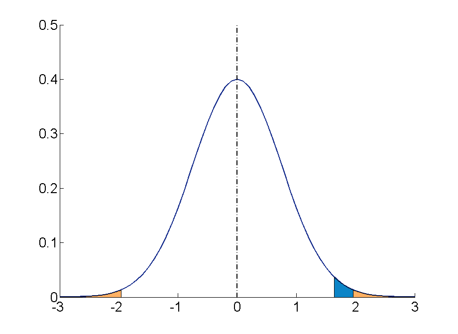
Step 4 : Your sample score of 27 needs to be converted into a Z value. To calculate Z = (27-19)/4= 2 ( check the Converting into Z scores section if you need to review how to do this process)
Step 5 : A ‘Z’ score of 2 is more extreme than the cut off Z of +1.96 (see figure above). The result is significant and, thus, the null hypothesis is rejected.
You can find more examples here:
- Statistics (RMIT Learning Lab)
Some commonly used statistical techniques
Correlation analysis, multiple regression.
- Analysis of variance
Chi-square test for independence
Correlation analysis explores the association between variables . The purpose of correlational analysis is to discover whether there is a relationship between variables, which is unlikely to occur by sampling error. The null hypothesis is that there is no relationship between the two variables. Correlation analysis provides information about:
- The direction of the relationship: positive or negative- given by the sign of the correlation coefficient.
- The strength or magnitude of the relationship between the two variables- given by the correlation coefficient, which varies from 0 (no relationship between the variables) to 1 (perfect relationship between the variables).
- Direction of the relationship.
A positive correlation indicates that high scores on one variable are associated with high scores on the other variable; low scores on one variable are associated with low scores on the second variable . For instance, in the figure below, higher scores on negative affect are associated with higher scores on perceived stress

A negative correlation indicates that high scores on one variable are associated with low scores on the other variable. The graph shows that a person who scores high on perceived stress will probably score low on mastery. The slope of the graph is downwards- as it moves to the right. In the figure below, higher scores on mastery are associated with lower scores on perceived stress.

Fig 2. Negative correlation between two variables. Adapted from Pallant, J. (2013). SPSS survival manual: A step by step guide to data analysis using IBM SPSS (5th ed.). Sydney, Melbourne, Auckland, London: Allen & Unwin
2. The strength or magnitude of the relationship
The strength of a linear relationship between two variables is measured by a statistic known as the correlation coefficient , which varies from 0 to -1, and from 0 to +1. There are several correlation coefficients; the most widely used are Pearson’s r and Spearman’s rho. The strength of the relationship is interpreted as follows:
- Small/weak: r= .10 to .29
- Medium/moderate: r= .30 to .49
- Large/strong: r= .50 to 1
It is important to note that correlation analysis does not imply causality. Correlation is used to explore the association between variables, however, it does not indicate that one variable causes the other. The correlation between two variables could be due to the fact that a third variable is affecting the two variables.
Multiple regression is an extension of correlation analysis. Multiple regression is used to explore the relationship between one dependent variable and a number of independent variables or predictors . The purpose of a multiple regression model is to predict values of a dependent variable based on the values of the independent variables or predictors. For example, a researcher may be interested in predicting students’ academic success (e.g. grades) based on a number of predictors, for example, hours spent studying, satisfaction with studies, relationships with peers and lecturers.
A multiple regression model can be conducted using statistical software (e.g. SPSS). The software will test the significance of the model (i.e. does the model significantly predicts scores on the dependent variable using the independent variables introduced in the model?), how much of the variance in the dependent variable is explained by the model, and the individual contribution of each independent variable.
Example of multiple regression model

From Dunn et al. (2014). Influence of academic self-regulation, critical thinking, and age on online graduate students' academic help-seeking.
In this model, help-seeking is the dependent variable; there are three independent variables or predictors. The coefficients show the direction (positive or negative) and magnitude of the relationship between each predictor and the dependent variable. The model was statistically significant and predicted 13.5% of the variance in help-seeking.
t-Tests are employed to compare the mean score on some continuous variable for two groups . The null hypothesis to be tested is there are no differences between the two groups (e.g. anxiety scores for males and females are not different).
If the significance value of the t-test is equal or less than .05, there is a significant difference in the mean scores on the variable of interest for each of the two groups. If the value is above .05, there is no significant difference between the groups.
t-Tests can be employed to compare the mean scores of two different groups (independent-samples t-test ) or to compare the same group of people on two different occasions ( paired-samples t-test) .
In addition to assessing whether the difference between the two groups is statistically significant, it is important to consider the effect size or magnitude of the difference between the groups. The effect size is given by partial eta squared (proportion of variance of the dependent variable that is explained by the independent variable) and Cohen’s d (difference between groups in terms of standard deviation units).
In this example, an independent samples t-test was conducted to assess whether males and females differ in their perceived anxiety levels. The significance of the test is .004. Since this value is less than .05, we can conclude that there is a statistically significant difference between males and females in their perceived anxiety levels.

Whilst t-tests compare the mean score on one variable for two groups, analysis of variance is used to test more than two groups . Following the previous example, analysis of variance would be employed to test whether there are differences in anxiety scores for students from different disciplines.
Analysis of variance compare the variance (variability in scores) between the different groups (believed to be due to the independent variable) with the variability within each group (believed to be due to chance). An F ratio is calculated; a large F ratio indicates that there is more variability between the groups (caused by the independent variable) than there is within each group (error term). A significant F test indicates that we can reject the null hypothesis; i.e. that there is no difference between the groups.
Again, effect size statistics such as Cohen’s d and eta squared are employed to assess the magnitude of the differences between groups.
In this example, we examined differences in perceived anxiety between students from different disciplines. The results of the Anova Test show that the significance level is .005. Since this value is below .05, we can conclude that there are statistically significant differences between students from different disciplines in their perceived anxiety levels.

Chi-square test for independence is used to explore the relationship between two categorical variables. Each variable can have two or more categories.
For example, a researcher can use a Chi-square test for independence to assess the relationship between study disciplines (e.g. Psychology, Business, Education,…) and help-seeking behaviour (Yes/No). The test compares the observed frequencies of cases with the values that would be expected if there was no association between the two variables of interest. A statistically significant Chi-square test indicates that the two variables are associated (e.g. Psychology students are more likely to seek help than Business students). The effect size is assessed using effect size statistics: Phi and Cramer’s V .
In this example, a Chi-square test was conducted to assess whether males and females differ in their help-seeking behaviour (Yes/No). The crosstabulation table shows the percentage of males of females who sought/didn't seek help. The table 'Chi square tests' shows the significance of the test (Pearson Chi square asymp sig: .482). Since this value is above .05, we conclude that there is no statistically significant difference between males and females in their help-seeking behaviour.

- << Previous: Probability and the normal distribution
- Next: Statistical techniques >>
Hypothesis Testing ( CIE A Level Maths: Probability & Statistics 2 )
Revision note.

Language of Hypothesis Testing
What is a hypothesis test.
- A hypothesis test uses a sample of data in an experiment to test a statement made about the value of a population parameter
- A hypothesis test is used when the value of the assumed population parameter is questioned
- The hypothesis test will look at the which outcomes are unlikely to occur if assumed population parameter is true
- The probability found will be compared against a given significance level to determine whether there is evidence to believe that the assumed population parameter is not true
What are the key terms used in statistical hypothesis testing?
- Every hypothesis test must begin with a clear null hypothesis (what we believe to already be true) and alternative hypothesis (how we believe the data pattern or probability distribution might have changed)
- One example of a population parameter is the probability, p of an event occurring
- Another example is the mean of a population
- The null hypothesis is denoted H 0 and sets out the assumed population parameter given that no change has happened
- The alternative hypothesis is denoted H 1 and sets out how we think the population parameter could have changed
- When a hypothesis test is carried out, the null hypothesis is assumed to be true and this assumption will either be accepted or rejected
- A hypothesis test could be a one-tailed test or a two-tailed test
- The null hypothesis will always be H 0 : θ = ...
- The alternative hypothesis, H 1 will be H 1 : θ > ... or H 1 : θ < ...
- The alternative hypothesis, H 1 will be H 1 : θ ≠ ...
- It is important to read the wording of the question carefully to decide whether your hypothesis test should be one-tailed or two-tailed
- A sample of data is a subset of data taken from the population
- The observed value is a numerical value calculated from the of data
- Any probability smaller than the significance level would suggest that the event is unlikely to have happened by chance
- The significance level must be set before the hypothesis test is carried out
- The significance level will usually be 1%, 5% or 10%, however it may vary
Worked example
A hypothesis test is carried out at the 5% level of significance to test if a normal coin is fair or not.

Make sure you read the question carefully to determine whether the test you are carrying out is for a one-tailed or a two-tailed test.
Critical Regions
How do we decide whether to reject or accept the null hypothesis.
- The critical region is the range of values that the observed value could take which will lead to the null hypothesis being rejected
- It is the least extreme value that would lead to the rejection of the null hypothesis
- The critical value is determined by the significance level
- In a two-tailed test the significance level is halved and both the upper and the lower tails are tested
- This probability will be known as the actual significance level
- The actual significance level is the probability of incorrectly rejecting the null hypothesis
- Finding the critical region will be different for a two-tailed test than it is for a one-tailed test
Do we always need to find the critical region?
- It allows you to see how far the observed value is from the critical value and make decisions about whether further testing is necessary
- In some cases a hypothesis test can be carried out without finding the critical region
- If the test is looking for a decrease then extreme values are smaller than the observed value, so find the probability of less than or equal to the observed value
- If the test is looking for an increase then extreme values are bigger than the observed value, so find the probability of greater than or equal to the observed value
- This probability is called the " p-value "
- In a two-tailed test it is common to half the significance level and compare this with the probability found in one of the tails
For the following situations, state at the 1% and 5% significance levels whether the null hypothesis should be rejected or not.

Conclusions of Hypothesis Testing
How is a hypothesis test carried out.
- There are a number of ways that a hypothesis test can be carried out for different models, however the following steps should form the base for your test:
- Step 1. Define the test statistic and population parameter
- Step 2. Write the null and alternative hypotheses clearly
- Step 3. Calculate the critical value(s) or the necessary probability for the test
- Step 4. Compare the observed value with the critical value(s) or the probability with the significance level
- Step 5. Decide whether there is enough evidence to reject H 0 or whether it has to be accepted
- Step 6. Write a conclusion in context
How should a conclusion be written for a hypothesis test?
- Your conclusion must be written in the context of the question
- If rejecting the null hypothesis your conclusion should state that there is sufficient evidence to suggest the alternative hypothesis is true at this level of significance
- If accepting the null hypothesis your conclusion should state that there is not enough evidence to suggest the alternative hypothesis is true at this level of significance
- There is a chance that the test has led to an incorrect conclusion
- The outcome is dependent on the sample, a different sample might lead to a different outcome
- You should not state whether this change is an increase or decrease
A teacher carried out a hypothesis test at the 10% significance level to test if her students perform better in exams after using a new revision technique. Under the null hypothesis she calculates the probability that a value will be at least as extreme as the observed value to be 0.09142. Write a conclusion for her hypothesis test.

- It is best to use the exact wording from the question when writing your conclusion for the hypothesis test, do not be afraid to sound repetitive.
You've read 0 of your 10 free revision notes
Get unlimited access.
to absolutely everything:
- Downloadable PDFs
- Unlimited Revision Notes
- Topic Questions
- Past Papers
- Model Answers
- Videos (Maths and Science)
Join the 100,000 + Students that ❤️ Save My Exams
the (exam) results speak for themselves:
Did this page help you?
Author: Amber
Amber gained a first class degree in Mathematics & Meteorology from the University of Reading before training to become a teacher. She is passionate about teaching, having spent 8 years teaching GCSE and A Level Mathematics both in the UK and internationally. Amber loves creating bright and informative resources to help students reach their potential.
Pardon Our Interruption
As you were browsing something about your browser made us think you were a bot. There are a few reasons this might happen:
- You've disabled JavaScript in your web browser.
- You're a power user moving through this website with super-human speed.
- You've disabled cookies in your web browser.
- A third-party browser plugin, such as Ghostery or NoScript, is preventing JavaScript from running. Additional information is available in this support article .
To regain access, please make sure that cookies and JavaScript are enabled before reloading the page.
Information
- Author Services
Initiatives
You are accessing a machine-readable page. In order to be human-readable, please install an RSS reader.
All articles published by MDPI are made immediately available worldwide under an open access license. No special permission is required to reuse all or part of the article published by MDPI, including figures and tables. For articles published under an open access Creative Common CC BY license, any part of the article may be reused without permission provided that the original article is clearly cited. For more information, please refer to https://www.mdpi.com/openaccess .
Feature papers represent the most advanced research with significant potential for high impact in the field. A Feature Paper should be a substantial original Article that involves several techniques or approaches, provides an outlook for future research directions and describes possible research applications.
Feature papers are submitted upon individual invitation or recommendation by the scientific editors and must receive positive feedback from the reviewers.
Editor’s Choice articles are based on recommendations by the scientific editors of MDPI journals from around the world. Editors select a small number of articles recently published in the journal that they believe will be particularly interesting to readers, or important in the respective research area. The aim is to provide a snapshot of some of the most exciting work published in the various research areas of the journal.
Original Submission Date Received: .
- Active Journals
- Find a Journal
- Proceedings Series
- For Authors
- For Reviewers
- For Editors
- For Librarians
- For Publishers
- For Societies
- For Conference Organizers
- Open Access Policy
- Institutional Open Access Program
- Special Issues Guidelines
- Editorial Process
- Research and Publication Ethics
- Article Processing Charges
- Testimonials
- Preprints.org
- SciProfiles
- Encyclopedia
Article Menu

- Subscribe SciFeed
- Recommended Articles
- Google Scholar
- on Google Scholar
- Table of Contents
Find support for a specific problem in the support section of our website.
Please let us know what you think of our products and services.
Visit our dedicated information section to learn more about MDPI.
JSmol Viewer
Review about the permutation approach in hypothesis testing.

Share and Cite
Bonnini, S.; Assegie, G.M.; Trzcinska, K. Review about the Permutation Approach in Hypothesis Testing. Mathematics 2024 , 12 , 2617. https://doi.org/10.3390/math12172617
Bonnini S, Assegie GM, Trzcinska K. Review about the Permutation Approach in Hypothesis Testing. Mathematics . 2024; 12(17):2617. https://doi.org/10.3390/math12172617
Bonnini, Stefano, Getnet Melak Assegie, and Kamila Trzcinska. 2024. "Review about the Permutation Approach in Hypothesis Testing" Mathematics 12, no. 17: 2617. https://doi.org/10.3390/math12172617
Article Metrics
Article access statistics, further information, mdpi initiatives, follow mdpi.
Subscribe to receive issue release notifications and newsletters from MDPI journals
Testing an hypothesis of hybrid zone movement for toads in France
- Naturalis Biodiversity Center
- Leiden University
- University of Sheffield
- University of Gothenburg
- University of California, Los Angeles
Research output : Contribution to journal › Article › peer-review
Hybrid zone movement may result in substantial unidirectional introgression of selectively neutral material from the local to the advancing species, leaving a genetic footprint. This genetic footprint is represented by a trail of asymmetric tails and displaced cline centres in the wake of the moving hybrid zone. A peak of admixture linkage disequilibrium is predicted to exist ahead of the centre of the moving hybrid zone. We test these predictions of the movement hypothesis in a hybrid zone between common (Bufo bufo) and spined toads (B. spinosus), using 31 nuclear and one mtDNA SNPs along a transect in the northwest of France. Average effective selection in Bufo hybrids is low and clines vary in shape and centre. A weak pattern of asymmetric introgression is inferred from cline discordance of seven nuclear markers. The dominant direction of gene flow is from B. spinosus to B. bufo and is in support of southward movement of the hybrid zone. Conversely, a peak of admixture linkage disequilibrium north of the hybrid zone suggests northward movement. These contrasting results can be explained by reproductive isolation of the B. spinosus and B. bufo gene pools at the southern (B. spinosus) side of the hybrid zone. The joint occurrence of asymmetric introgression and admixture linkage disequilibrium can also be explained by the combination of low dispersal and random genetic drift due to low effective population sizes.
| Original language | English |
|---|---|
| Pages (from-to) | 1070-1083 |
| Number of pages | 14 |
| Journal | |
| Volume | 28 |
| Issue number | 5 |
| DOIs | |
| Publication status | Published - 2019 Mar |
| Externally published | Yes |
Bibliographical note
Free keywords.
- admixture linkage disequilibrium
- asymmetric reproductive isolation
- Bufo spinosus
- cline coupling
- hybrid zone movement
Access to Document
- 10.1111/mec.15005
Fingerprint
- France Earth and Planetary Sciences 100%
- Anura Agricultural and Biological Sciences 100%
- Movement Medicine and Dentistry 100%
- Linkage Earth and Planetary Sciences 37%
- Admixture Earth and Planetary Sciences 37%
- Linkage Disequilibrium Agricultural and Biological Sciences 37%
- Introgression Agricultural and Biological Sciences 37%
- Bufo Agricultural and Biological Sciences 37%
T1 - Testing an hypothesis of hybrid zone movement for toads in France
AU - van Riemsdijk, Isolde
AU - Butlin, Roger K.
AU - Wielstra, Ben
AU - Arntzen, Jan W.
N1 - Publisher Copyright: © 2019 John Wiley & Sons Ltd
PY - 2019/3
Y1 - 2019/3
N2 - Hybrid zone movement may result in substantial unidirectional introgression of selectively neutral material from the local to the advancing species, leaving a genetic footprint. This genetic footprint is represented by a trail of asymmetric tails and displaced cline centres in the wake of the moving hybrid zone. A peak of admixture linkage disequilibrium is predicted to exist ahead of the centre of the moving hybrid zone. We test these predictions of the movement hypothesis in a hybrid zone between common (Bufo bufo) and spined toads (B. spinosus), using 31 nuclear and one mtDNA SNPs along a transect in the northwest of France. Average effective selection in Bufo hybrids is low and clines vary in shape and centre. A weak pattern of asymmetric introgression is inferred from cline discordance of seven nuclear markers. The dominant direction of gene flow is from B. spinosus to B. bufo and is in support of southward movement of the hybrid zone. Conversely, a peak of admixture linkage disequilibrium north of the hybrid zone suggests northward movement. These contrasting results can be explained by reproductive isolation of the B. spinosus and B. bufo gene pools at the southern (B. spinosus) side of the hybrid zone. The joint occurrence of asymmetric introgression and admixture linkage disequilibrium can also be explained by the combination of low dispersal and random genetic drift due to low effective population sizes.
AB - Hybrid zone movement may result in substantial unidirectional introgression of selectively neutral material from the local to the advancing species, leaving a genetic footprint. This genetic footprint is represented by a trail of asymmetric tails and displaced cline centres in the wake of the moving hybrid zone. A peak of admixture linkage disequilibrium is predicted to exist ahead of the centre of the moving hybrid zone. We test these predictions of the movement hypothesis in a hybrid zone between common (Bufo bufo) and spined toads (B. spinosus), using 31 nuclear and one mtDNA SNPs along a transect in the northwest of France. Average effective selection in Bufo hybrids is low and clines vary in shape and centre. A weak pattern of asymmetric introgression is inferred from cline discordance of seven nuclear markers. The dominant direction of gene flow is from B. spinosus to B. bufo and is in support of southward movement of the hybrid zone. Conversely, a peak of admixture linkage disequilibrium north of the hybrid zone suggests northward movement. These contrasting results can be explained by reproductive isolation of the B. spinosus and B. bufo gene pools at the southern (B. spinosus) side of the hybrid zone. The joint occurrence of asymmetric introgression and admixture linkage disequilibrium can also be explained by the combination of low dispersal and random genetic drift due to low effective population sizes.
KW - admixture linkage disequilibrium
KW - asymmetric reproductive isolation
KW - Bufo bufo
KW - Bufo spinosus
KW - cline coupling
KW - hybrid zone movement
U2 - 10.1111/mec.15005
DO - 10.1111/mec.15005
M3 - Article
C2 - 30609055
AN - SCOPUS:85063687723
SN - 0962-1083
JO - Molecular Ecology
JF - Molecular Ecology
COMMENTS
Table of contents. Step 1: State your null and alternate hypothesis. Step 2: Collect data. Step 3: Perform a statistical test. Step 4: Decide whether to reject or fail to reject your null hypothesis. Step 5: Present your findings. Other interesting articles. Frequently asked questions about hypothesis testing.
8.2 FOUR STEPS TO HYPOTHESIS TESTING The goal of hypothesis testing is to determine the likelihood that a population parameter, such as the mean, is likely to be true. In this section, we describe the four steps of hypothesis testing that were briefly introduced in Section 8.1: Step 1: State the hypotheses. Step 2: Set the criteria for a decision.
A hypothesis test consists of five steps: 1. State the hypotheses. State the null and alternative hypotheses. These two hypotheses need to be mutually exclusive, so if one is true then the other must be false. 2. Determine a significance level to use for the hypothesis. Decide on a significance level.
Important Notes on Hypothesis Testing. Hypothesis testing is a technique that is used to verify whether the results of an experiment are statistically significant. It involves the setting up of a null hypothesis and an alternate hypothesis.
Chapter 5 Hypothesis Testing. Chapter 5Hypothesis TestingA second type of statistical inf. rence is hypothesis testing. Here, rather than use ei-ther a point (or interval) estimate from a random sample to approximate a population parameter, hypothesis testing uses point estimate to decide which of two hypotheses (guesses.
Note the asymmetry between the null and alternative hypotheses. This asymmetry is due to the fact that we assume the null hypothesis, in a sense, and then see if there is sufficient evidence in \(\bs{x}\) to overturn this assumption in favor of the alternative. An hypothesis test is a statistical analogy to proof by contradiction, in a sense.
Alternative Hypothesis: The alternative hypothesis is a statement that suggests there is a statistically significant effect or difference in a given situation, opposing the null hypothesis. This hypothesis typically predicts the outcome researchers expect to find when conducting an experiment or analysis, playing a critical role in hypothesis testing by guiding the direction of research and ...
In binary hypothesis testing problems, we'll often be presented with two choices which we call hypotheses, and we'll have to decide whether to pick one or the other. The hypotheses are represented by H₀ and H₁ and are called null and alternate hypotheses respectively. In hypothesis testing, we either reject or accept the null hypothesis.
Hypothesis testing is a method of statistical inference that considers the null hypothesis H ₀ vs. the alternative hypothesis H a, where we are typically looking to assess evidence against H ₀. Such a test is used to compare data sets against one another, or compare a data set against some external standard. The former being a two sample ...
In reviewing hypothesis tests, we start first with the general idea. Then, we keep returning to the basic procedures of hypothesis testing, each time adding a little more detail. ... blood spots, hair samples, carpet fibers, shoe prints, ransom notes, and handwriting samples — with the hopes of finding "sufficient evidence" to make the ...
The intent of hypothesis testing is formally examine two opposing conjectures (hypotheses), H0 and HA. These two hypotheses are mutually exclusive and exhaustive so that one is true to the exclusion of the other. We accumulate evidence - collect and analyze sample information - for the purpose of determining which of the two hypotheses is true ...
This tests whether the population parameter is equal to, versus less than, some specific value. Ho: μ = 12 vs. H1: μ < 12. The critical region is in the left tail and the critical value is a negative value that defines the rejection zone. Figure 3.1.3 3.1. 3: The rejection zone for a left-sided hypothesis test.
A hypothesis test is carried out at the 5% level of significance to test if a normal coin is fair or not. (i) Describe what the population parameter could be for the hypothesis test. (ii) State whether the hypothesis test should be a one-tailed test or a two-tailed test, give a reason for your answer. (iii)
Steps in Hypothesis Testing: Book lists 9 - I use 5. You can see it is the same process. For each test we learn, we will see di erences in assumptions, formulas, etc., but the basic test setup is the same. We will learn about test statistics and p-values next week. Right now I want you to see where the hypothesis setup and choosing t in the ...
Effect size. Significance tests inform us about the likelihood of a meaningful difference between groups, but they don't always tell us the magnitude of that difference. Because any difference will become "significant" with an arbitrarily large sample, it's important to quantify the effect size that you observe.
o the sampling distribution un. r 0.The hypothesis testing recipeThe basic id. is:If the true parameter was 0...then T (Y) should look like it c. e from f(Y j 0).We compare the observed T (Y) to the sampling distribution under 0.If the observed T (Y) is unlik. ly under the sampling distribution given 0, we reject the null hy.
Plan for these notes I Describing a random variable I Expected value and variance I Probability density function I Normal distribution I Reading the table of the standard normal I Hypothesis testing on the mean I The basic intuition I Level of signi cance, p-value and power of a test I An example Michele Pi er (LSE)Hypothesis Testing for BeginnersAugust, 2011 3 / 53
9 Hypothesis Tests. (Ch 9.1-9.3, 9.5-9.9) Statistical hypothesis: a claim about the value of a parameter or population characteristic. Examples: H: μ = 75 cents, where μ is the true population average of daily per-student candy+soda expenses in US high schools. H: p < .10, where p is the population proportion of defective helmets for a given ...
If the biologist set her significance level \(\alpha\) at 0.05 and used the critical value approach to conduct her hypothesis test, she would reject the null hypothesis if her test statistic t* were less than -1.6939 (determined using statistical software or a t-table):s-3-3. Since the biologist's test statistic, t* = -4.60, is less than -1.6939, the biologist rejects the null hypothesis.
Case1: Population is normally or approximately normally distributed with known or unknown variance (sample size n may be small or large), Case 2: Population is not normal with known or unknown variance (n is large i.e. n≥30). 3.Hypothesis: we have three cases. Case I : H0: μ=μ0 HA: μ μ0. e.g. we want to test that the population mean is ...
The process of testing hypotheses follows a simple four-step procedure. This process will be what we use for the remained of the textbook and course, and though the hypothesis and statistics we use will change, this process will not. Step 1: State the Hypotheses Your hypotheses are the first thing you need to lay out. Otherwise, there is ...
Hypothesis testing is a statistical method used to determine if there is enough evidence in a sample data to draw conclusions about a population. It involves formulating two competing hypotheses, the null hypothesis (H0) and the alternative hypothesis (Ha), and then collecting data to assess the evidence. ...
Note: The p-value is the probability of obtaining a test statistic as extreme as, or more extreme than, the one observed in the sample, assuming the null hypothesis is true. To determine p-value for hypothesis testing, we typically refer to a statistical distribution table , such as the normal distribution or t-distribution tables based on.
The purpose of hypothesis testing is to test whether the null hypothesis (there is no difference, no effect) can be rejected or approved. If the null hypothesis is rejected, then the research hypothesis can be accepted. ... It is important to note that correlation analysis does not imply causality. Correlation is used to explore the association ...
A hypothesis test uses a sample of data in an experiment to test a statement made about the value of a population parameter. A hypothesis test is used when the value of the assumed population parameter is questioned. The hypothesis test will look at the which outcomes are unlikely to occur if assumed population parameter is true.
ii. Hypothesis testing is a procedure based on sample evidence and probability theory to decide whether the hypothesis is a reasonable statement. iii. We call a statement about the value of a population parameter a hypothesis. A. (i), (ii), and (iii) are all correct statements. B. (i) is a correct statement but not (ii) or (iii). C.
Today, permutation tests represent a powerful and increasingly widespread tool of statistical inference for hypothesis-testing problems. To the best of our knowledge, a review of the application of permutation tests for complex data in practical data analysis for hypothesis testing is missing. In particular, it is essential to review the application of permutation tests in two-sample or multi ...
A peak of admixture linkage disequilibrium is predicted to exist ahead of the centre of the moving hybrid zone. We test these predictions of the movement hypothesis in a hybrid zone between common (Bufo bufo) and spined toads (B. spinosus), using 31 nuclear and one mtDNA SNPs along a transect in the northwest of France.