
Want to create or adapt books like this? Learn more about how Pressbooks supports open publishing practices.

Factorial Designs
41 setting up a factorial experiment, learning objectives.
- Explain why researchers often include multiple independent variables in their studies.
- Define factorial design, and use a factorial design table to represent and interpret simple factorial designs.
Just as it is common for studies in psychology to include multiple levels of a single independent variable (placebo, new drug, old drug), it is also common for them to include multiple independent variables. Schnall and her colleagues studied the effect of both disgust and private body consciousness in the same study. Researchers’ inclusion of multiple independent variables in one experiment is further illustrated by the following actual titles from various professional journals:
- The Effects of Temporal Delay and Orientation on Haptic Object Recognition
- Opening Closed Minds: The Combined Effects of Intergroup Contact and Need for Closure on Prejudice
- Effects of Expectancies and Coping on Pain-Induced Intentions to Smoke
- The Effect of Age and Divided Attention on Spontaneous Recognition
- The Effects of Reduced Food Size and Package Size on the Consumption Behavior of Restrained and Unrestrained Eaters
Just as including multiple levels of a single independent variable allows one to answer more sophisticated research questions, so too does including multiple independent variables in the same experiment. For example, instead of conducting one study on the effect of disgust on moral judgment and another on the effect of private body consciousness on moral judgment, Schnall and colleagues were able to conduct one study that addressed both questions. But including multiple independent variables also allows the researcher to answer questions about whether the effect of one independent variable depends on the level of another. This is referred to as an interaction between the independent variables. Schnall and her colleagues, for example, observed an interaction between disgust and private body consciousness because the effect of disgust depended on whether participants were high or low in private body consciousness. As we will see, interactions are often among the most interesting results in psychological research.
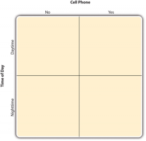
By far the most common approach to including multiple independent variables (which are often called factors) in an experiment is the factorial design. In a factorial design , each level of one independent variable is combined with each level of the others to produce all possible combinations. Each combination, then, becomes a condition in the experiment. Imagine, for example, an experiment on the effect of cell phone use (yes vs. no) and time of day (day vs. night) on driving ability. This is shown in the factorial design table in Figure 9.1. The columns of the table represent cell phone use, and the rows represent time of day. The four cells of the table represent the four possible combinations or conditions: using a cell phone during the day, not using a cell phone during the day, using a cell phone at night, and not using a cell phone at night. This particular design is referred to as a 2 × 2 (read “two-by-two”) factorial design because it combines two variables, each of which has two levels.
If one of the independent variables had a third level (e.g., using a handheld cell phone, using a hands-free cell phone, and not using a cell phone), then it would be a 3 × 2 factorial design, and there would be six distinct conditions. Notice that the number of possible conditions is the product of the numbers of levels. A 2 × 2 factorial design has four conditions, a 3 × 2 factorial design has six conditions, a 4 × 5 factorial design would have 20 conditions, and so on. Also notice that each number in the notation represents one factor, one independent variable. So by looking at how many numbers are in the notation, you can determine how many independent variables there are in the experiment. 2 x 2, 3 x 3, and 2 x 3 designs all have two numbers in the notation and therefore all have two independent variables. The numerical value of each of the numbers represents the number of levels of each independent variable. A 2 means that the independent variable has two levels, a 3 means that the independent variable has three levels, a 4 means it has four levels, etc. To illustrate a 3 x 3 design has two independent variables, each with three levels, while a 2 x 2 x 2 design has three independent variables, each with two levels.
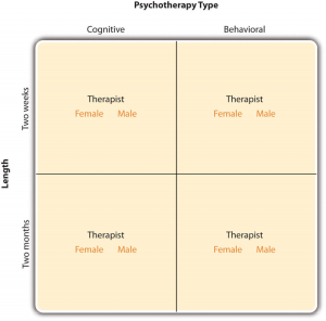
In principle, factorial designs can include any number of independent variables with any number of levels. For example, an experiment could include the type of psychotherapy (cognitive vs. behavioral), the length of the psychotherapy (2 weeks vs. 2 months), and the sex of the psychotherapist (female vs. male). This would be a 2 × 2 × 2 factorial design and would have eight conditions. Figure 9.2 shows one way to represent this design. In practice, it is unusual for there to be more than three independent variables with more than two or three levels each. This is for at least two reasons: For one, the number of conditions can quickly become unmanageable. For example, adding a fourth independent variable with three levels (e.g., therapist experience: low vs. medium vs. high) to the current example would make it a 2 × 2 × 2 × 3 factorial design with 24 distinct conditions. Second, the number of participants required to populate all of these conditions (while maintaining a reasonable ability to detect a real underlying effect) can render the design unfeasible (for more information, see the discussion about the importance of adequate statistical power in Chapter 13). As a result, in the remainder of this section, we will focus on designs with two independent variables. The general principles discussed here extend in a straightforward way to more complex factorial designs.
Assigning Participants to Conditions
Recall that in a simple between-subjects design, each participant is tested in only one condition. In a simple within-subjects design, each participant is tested in all conditions. In a factorial experiment, the decision to take the between-subjects or within-subjects approach must be made separately for each independent variable. In a between-subjects factorial design , all of the independent variables are manipulated between subjects. For example, all participants could be tested either while using a cell phone or while not using a cell phone and either during the day or during the night. This would mean that each participant would be tested in one and only one condition. In a within-subjects factorial design, all of the independent variables are manipulated within subjects. All participants could be tested both while using a cell phone and while not using a cell phone and both during the day and during the night. This would mean that each participant would need to be tested in all four conditions. The advantages and disadvantages of these two approaches are the same as those discussed in Chapter 5. The between-subjects design is conceptually simpler, avoids order/carryover effects, and minimizes the time and effort of each participant. The within-subjects design is more efficient for the researcher and controls extraneous participant variables.
Since factorial designs have more than one independent variable, it is also possible to manipulate one independent variable between subjects and another within subjects. This is called a mixed factorial design . For example, a researcher might choose to treat cell phone use as a within-subjects factor by testing the same participants both while using a cell phone and while not using a cell phone (while counterbalancing the order of these two conditions). But they might choose to treat time of day as a between-subjects factor by testing each participant either during the day or during the night (perhaps because this only requires them to come in for testing once). Thus each participant in this mixed design would be tested in two of the four conditions.
Regardless of whether the design is between subjects, within subjects, or mixed, the actual assignment of participants to conditions or orders of conditions is typically done randomly.
Non-Manipulated Independent Variables
In many factorial designs, one of the independent variables is a non-manipulated independent variable . The researcher measures it but does not manipulate it. The study by Schnall and colleagues is a good example. One independent variable was disgust, which the researchers manipulated by testing participants in a clean room or a messy room. The other was private body consciousness, a participant variable which the researchers simply measured. Another example is a study by Halle Brown and colleagues in which participants were exposed to several words that they were later asked to recall (Brown, Kosslyn, Delamater, Fama, & Barsky, 1999) [1] . The manipulated independent variable was the type of word. Some were negative health-related words (e.g., tumor, coronary ), and others were not health related (e.g., election, geometry ). The non-manipulated independent variable was whether participants were high or low in hypochondriasis (excessive concern with ordinary bodily symptoms). The result of this study was that the participants high in hypochondriasis were better than those low in hypochondriasis at recalling the health-related words, but they were no better at recalling the non-health-related words.
Such studies are extremely common, and there are several points worth making about them. First, non-manipulated independent variables are usually participant variables (private body consciousness, hypochondriasis, self-esteem, gender, and so on), and as such, they are by definition between-subjects factors. For example, people are either low in hypochondriasis or high in hypochondriasis; they cannot be tested in both of these conditions. Second, such studies are generally considered to be experiments as long as at least one independent variable is manipulated, regardless of how many non-manipulated independent variables are included. Third, it is important to remember that causal conclusions can only be drawn about the manipulated independent variable. For example, Schnall and her colleagues were justified in concluding that disgust affected the harshness of their participants’ moral judgments because they manipulated that variable and randomly assigned participants to the clean or messy room. But they would not have been justified in concluding that participants’ private body consciousness affected the harshness of their participants’ moral judgments because they did not manipulate that variable. It could be, for example, that having a strict moral code and a heightened awareness of one’s body are both caused by some third variable (e.g., neuroticism). Thus it is important to be aware of which variables in a study are manipulated and which are not.
Non-Experimental Studies With Factorial Designs
Thus far we have seen that factorial experiments can include manipulated independent variables or a combination of manipulated and non-manipulated independent variables. But factorial designs can also include only non-manipulated independent variables, in which case they are no longer experiments but are instead non-experimental in nature. Consider a hypothetical study in which a researcher simply measures both the moods and the self-esteem of several participants—categorizing them as having either a positive or negative mood and as being either high or low in self-esteem—along with their willingness to have unprotected sexual intercourse. This can be conceptualized as a 2 × 2 factorial design with mood (positive vs. negative) and self-esteem (high vs. low) as non-manipulated between-subjects factors. Willingness to have unprotected sex is the dependent variable.
Again, because neither independent variable in this example was manipulated, it is a non-experimental study rather than an experiment. (The similar study by MacDonald and Martineau [2002] [2] was an experiment because they manipulated their participants’ moods.) This is important because, as always, one must be cautious about inferring causality from non-experimental studies because of the directionality and third-variable problems. For example, an effect of participants’ moods on their willingness to have unprotected sex might be caused by any other variable that happens to be correlated with their moods.
- Brown, H. D., Kosslyn, S. M., Delamater, B., Fama, A., & Barsky, A. J. (1999). Perceptual and memory biases for health-related information in hypochondriacal individuals. Journal of Psychosomatic Research, 47 , 67–78. ↵
- MacDonald, T. K., & Martineau, A. M. (2002). Self-esteem, mood, and intentions to use condoms: When does low self-esteem lead to risky health behaviors? Journal of Experimental Social Psychology, 38 , 299–306. ↵
Experiments that include more than one independent variable in which each level of one independent variable is combined with each level of the others to produce all possible combinations.
Shows how each level of one independent variable is combined with each level of the others to produce all possible combinations in a factorial design.
All of the independent variables are manipulated between subjects.
A design which manipulates one independent variable between subjects and another within subjects.
An independent variable that is measured but is non-manipulated.
Research Methods in Psychology Copyright © 2019 by Rajiv S. Jhangiani, I-Chant A. Chiang, Carrie Cuttler, & Dana C. Leighton is licensed under a Creative Commons Attribution-NonCommercial-ShareAlike 4.0 International License , except where otherwise noted.
Share This Book

Factorial Design of Experiments
Learning outcomes.
After successfully completing the Module 4 Factorial Design of Experiments, students will be able to
- Explain the Factorial design of experiments
- Explain the data structure/layout of a factorial design of experiment
- Explain the coding systems used in a factorial design of experiment
- Calculate the main and the interaction effects
- Graphically represent the design and the analysis results, including the main effects and the interaction effects
- Develop the regression equations from the effects
- Perform the regression response surface analysis to produce the contour plot and the response surface
- Interpret the main and the interaction effects using the contour plot and the response surface
- Develop the ANOVA table from the effects
- Interpret the results in the context of the problem
What is a Factorial Design of Experiment?
The factorial design of experiment is described with examples in Video 1.
Video 1. Introduction to Factorial Design of Experiment DOE and the Main Effect Calculation Explained Example .
In a Factorial Design of Experiment, all possible combinations of the levels of a factor can be studied against all possible levels of other factors. Therefore, the factorial design of experiments is also called the crossed factor design of experiments . Due to the crossed nature of the levels, the factorial design of experiments can also be called the completely randomized design (CRD) of experiments . Therefore, the proper name for the factorial design of experiments would be completely randomized factorial design of experiments .
In an easy to understand study of human comfort, two levels of the temperature factor (or independent variable), including 0 O F and 75 O F; and two levels of the humidity factor, including 0% and 35% were studied with all possible combinations (Figure 1). Therefore, the four (2X2) possible treatment combinations, and their associated responses from human subjects (experimental units) are provided in Table 1.
Table 1. Data Structure/Layout of a Factorial Design of Experiment

Coding Systems for the Factor Levels in the Factorial Design of Experiment
As the factorial design is primarily used for screening variables, only two levels are enough. Often, coding the levels as (1) low/high, (2) -/+ or (3) -1/+1 is more convenient and meaningful than the actual level of the factors, especially for the designs and analyses of the factorial experiments. These coding systems are particularly useful in developing the methods in factorial and fractional factorial design of experiments. Moreover, general formula and methods can only be developed utilizing the coding system. Coding systems are also useful in response surface methodology. Often, coded levels produce smooth, meaningful and easy to understand contour plots and response surfaces. Moreover, especially in complex designs, the coded levels such as the low- and high-level of a factor are easier to understand.
How to graphically represent the design?
An example graphical representation of a factorial design of experiment is provided in Figure 1 .

Figure 1. Factorial Design of Experiments with two levels for each factor (independent variable, x). The response (dependent variable, y) is shown using the solid black circle with the associated response values.
How to calculate the main effects?
The calculation of the main effects from a factorial design of experiment is described with examples in Video 2 (both Video 1 and Video 2 are the same).
Video 2. Introduction to Factorial Design of Experiment DOE and the Main Effect Calculation Explained Example .
The average effect of the factor A (called the main effect of A) can be calculated from the average responses at the high level of A minus the average responses at the low level of A (Figure 2). When the main effect of A is calculated, all other factors are ignored assuming that we don’t have anything else other than the interested factor, which is A, the temperature factor.
Therefore, the main effect of the temperature factor can be calculated as A = (9+5)/2 - (2+0)/2 = 7-1 = 6. The calculation can be seen in figure 2.
= the average comfort increases by 6 on a scale of 0 (least comfortable) to 10 (most comfortable) if the temperature increases from 0- to 75-degree Fahrenheit.
Similarly, the main effect of B is calculated by ignoring all other factors assuming we don’t have anything else other than the interested factor, which is B, the humidity factor.
Therefore, the main effect of the humidity factor can be calculated as B= (2+9)/2- (5+0)/2=5.5-2.5=3. The calculation can be seen in figure 3.
= the average comfort increases by 3 on a scale of 0 (least comfortable) to 10 (most comfortable) if the relative humidity increases from 0 to 35 percent.

Figure 2. Graphical representation of the main effect of the temperature (factor A).

Figure 3. Graphical representation of the main effect of the humidity (factor B).
How to calculate the interaction effects?
The calculation of the interaction effects from a factorial design of experiment is provided in Video 3.
Video 3. How to calculate Two Factors Interaction Effect in Any Design of Experiments DOE Explained Examples .
In contrast to the main effects (the independent effect of a factor), in real world, factors (variables) may interact between each other to affect the responses. For an example, the temperature and the humidity may interact with each other to affect the human comfort.
At the low humidity level (0%), the comfort increases by 5 (=5-0) if the temperature increases from 0- to 75-degree Fahrenheit. However, at the high humidity level (35%), the comfort increases by 7 (=9-2) if the temperature increases form 0- to 75-degree Fahrenheit (Figure 4). Therefore, at different levels of the humidity factor, the changes in comfort are not the same even if the temperature change is same (from 0 to 75 degree). The effect of temperature (factor A) is different across the level of the factor B (humidity). This phenomenon is called the Interaction Effect , which is expressed by AB.
The average difference or change in comfort can be calculated as AB= (7-5)/2= 2/2=1.
= the change in comfort level increases by 1 more at the high level as compared to the low level of humidity (factor B) if the temperature (factor A) increase from the low level (0-degree) to the high level (75-degree).
Similarly, the interaction effect can be calculated for the humidity factor across the level of temperature factor as follows.
At the low level of A, effect of B = 2-0 = 2; at the high level of A, the effect of B = 9-5 = 4 (Figure 5). Therefore, the average difference or change in comfort can be calculated as AB= (4-2)/2= 2/2=1.
= the change in comfort level increases by 1 more at the high level as compared to the low level of temperature (factor A) if the humidity (factor B) increase from the low level (0 %) to the high level (35%).
The interaction effect is same whether it is calculated across the level of factor A or factor B.

Figure 4. Interaction effects of the temperature (factor A) and the humidity (factor B).

Figure 5. Interaction effects of the temperature (factor A) and the humidity (factor B).
What is a Strong or No/Absence of Interaction?
As the interaction effect is comparatively low or small in this example, the figure shows a slight or small interaction (Figure 4 & Figure 5). A strong interaction is depicted in Figure 6. No interaction effect would produce parallel lines shown in Figure 7.

Figure 6. Visualization of a strong interaction effect.

Figure 7. Visualization of no interaction effect.
How to develop the regression equation from the main and the interaction effects?
Video 4 demonstrates the process of developing regression equations from the effect estimates.
Video 4. How to Develop Regression using the Calculated Effects from a Factorial Design of Experiment .
For quantitative independent variables (factors), an estimated regression equation can be developed from the calculated main effects and the interaction effects. The full regression model with two factors (two level for each factor) with the interaction effect can be written as Equation 1.

How to estimate the regression coefficients from the main and the interaction effects.
Using the -1/+1 coding system (Figure 8), the average comfort level increases by 6 ((9+5-2-0)/2=6) if the temperature is increased by two units (-1 to 0 and then from 0 to +1). Therefore, for one unit increase of the temperature, the comfort level is increased by 3. As the estimate for the coefficients, beta for an example is the increase of the response for every one unit increase of the factor level, the estimated regression coefficient is calculated as one-half of the respective estimated effect.
The regression coefficient is one-half of the calculated effect. The regression constant is calculated by averaging all four responses. Therefore, the regression equation can be written as in Equation.

Figure 8. How to estimate the regression coefficients from the main and the interaction effects.
Video 5. Basic Response Surface Methodology RSM Factorial Design of Experiments DOE Explained With Examples .
The contour plot and the response surface representation of the regression
The contour plot and the response surface are visualized in Figure 9 & Figure 10, respectively. The comfort level increases as the temperature increase. However, the effect of humidity is not as obvious as the temperature as the estimated effect is 50% (1.5) as compared to the temperature (3). Moreover, near straight lines shows very little interaction between the temperature and the humidity to affect the human comfort.

Figure 9. Visualization of the contour plot for the effect of temperature and humidity on human comfort.

Figure 10. Visualization of the response surface for the effect of temperature and humidity on human comfort.
How to construct the ANOVA table from the main and the interaction effects?
Video 6 demonstrates the process of constructing the ANOVA table from the main and the interaction effects.
Video 6. How to Construct ANOVA Table from the Effect Estimates from the Factorial Design of Experiments DOE .
ANOVA table can be constructed using the calculated main and the interaction effects. Details will be discussed in the “Module 5: 2K factorial design of experiments.” For this particular example with only two independent variables (factors) having two levels for each factor without any replications, the sum of square is simply calculated as the square of the effects. For an example, the sum of square for the temperature variable (factor) is the square of the temperature effect of an increase in comfort level of 6, which is 36 (6 2 ). No experimental error can be calculated without replication. Therefore, the experimental error is zero (0) for this example. Therefore, the F-statistics and the p-value cannot be calculated for this example. The ANOVA table can be constructed as in Table 2.

*need replications (experimental error) to calculate these values
Table 2 ANOVA table from the calculated main and interaction effects
Practice Problem # 1
The effect of water and sunlight on the plant growth rate was measured on a scale of 0 (no growth) to 10 (highest level). Data is provided in Table 2.
- Draw the experimental diagram as in Figure 1.
- Calculate the main effect of factor A. Interpret the result in the context of the problem.
- Calculate the main effect of factor B. Interpret the result in the context of the problem.
- Calculate the interaction effect of factor AB. Interpret the result in the context of the problem.
- Produce the mean plots for the main and interaction effects.
- Produce the estimated regression equation.
- Construct the ANOVA table from the estimates.

Table 2. Factorial Design of Experiments Practice Example
2K Factorial Design of Experiments
Research Methods in Psychology
5. factorial designs ¶.
We have usually no knowledge that any one factor will exert its effects independently of all others that can be varied, or that its effects are particularly simply related to variations in these other factors. —Ronald Fisher
In Chapter 1 we briefly described a study conducted by Simone Schnall and her colleagues, in which they found that washing one’s hands leads people to view moral transgressions as less wrong [SBH08] . In a different but related study, Schnall and her colleagues investigated whether feeling physically disgusted causes people to make harsher moral judgments [SHCJ08] . In this experiment, they manipulated participants’ feelings of disgust by testing them in either a clean room or a messy room that contained dirty dishes, an overflowing wastebasket, and a chewed-up pen. They also used a self-report questionnaire to measure the amount of attention that people pay to their own bodily sensations. They called this “private body consciousness”. They measured their primary dependent variable, the harshness of people’s moral judgments, by describing different behaviors (e.g., eating one’s dead dog, failing to return a found wallet) and having participants rate the moral acceptability of each one on a scale of 1 to 7. They also measured some other dependent variables, including participants’ willingness to eat at a new restaurant. Finally, the researchers asked participants to rate their current level of disgust and other emotions. The primary results of this study were that participants in the messy room were in fact more disgusted and made harsher moral judgments than participants in the clean room—but only if they scored relatively high in private body consciousness.
The research designs we have considered so far have been simple—focusing on a question about one variable or about a statistical relationship between two variables. But in many ways, the complex design of this experiment undertaken by Schnall and her colleagues is more typical of research in psychology. Fortunately, we have already covered the basic elements of such designs in previous chapters. In this chapter, we look closely at how and why researchers combine these basic elements into more complex designs. We start with complex experiments—considering first the inclusion of multiple dependent variables and then the inclusion of multiple independent variables. Finally, we look at complex correlational designs.
5.1. Multiple Dependent Variables 
5.1.1. learning objectives ¶.
Explain why researchers often include multiple dependent variables in their studies.
Explain what a manipulation check is and when it would be included in an experiment.
Imagine that you have made the effort to find a research topic, review the research literature, formulate a question, design an experiment, obtain approval from teh relevant institutional review board (IRB), recruit research participants, and manipulate an independent variable. It would seem almost wasteful to measure a single dependent variable. Even if you are primarily interested in the relationship between an independent variable and one primary dependent variable, there are usually several more questions that you can answer easily by including multiple dependent variables.
5.1.2. Measures of Different Constructs 
Often a researcher wants to know how an independent variable affects several distinct dependent variables. For example, Schnall and her colleagues were interested in how feeling disgusted affects the harshness of people’s moral judgments, but they were also curious about how disgust affects other variables, such as people’s willingness to eat in a restaurant. As another example, researcher Susan Knasko was interested in how different odors affect people’s behavior [Kna92] . She conducted an experiment in which the independent variable was whether participants were tested in a room with no odor or in one scented with lemon, lavender, or dimethyl sulfide (which has a cabbage-like smell). Although she was primarily interested in how the odors affected people’s creativity, she was also curious about how they affected people’s moods and perceived health—and it was a simple enough matter to measure these dependent variables too. Although she found that creativity was unaffected by the ambient odor, she found that people’s moods were lower in the dimethyl sulfide condition, and that their perceived health was greater in the lemon condition.
When an experiment includes multiple dependent variables, there is again a possibility of carryover effects. For example, it is possible that measuring participants’ moods before measuring their perceived health could affect their perceived health or that measuring their perceived health before their moods could affect their moods. So the order in which multiple dependent variables are measured becomes an issue. One approach is to measure them in the same order for all participants—usually with the most important one first so that it cannot be affected by measuring the others. Another approach is to counterbalance, or systematically vary, the order in which the dependent variables are measured.
5.1.3. Manipulation Checks 
When the independent variable is a construct that can only be manipulated indirectly—such as emotions and other internal states—an additional measure of that independent variable is often included as a manipulation check. This is done to confirm that the independent variable was, in fact, successfully manipulated. For example, Schnall and her colleagues had their participants rate their level of disgust to be sure that those in the messy room actually felt more disgusted than those in the clean room.
Manipulation checks are usually done at the end of the procedure to be sure that the effect of the manipulation lasted throughout the entire procedure and to avoid calling unnecessary attention to the manipulation. Manipulation checks become especially important when the manipulation of the independent variable turns out to have no effect on the dependent variable. Imagine, for example, that you exposed participants to happy or sad movie music—intending to put them in happy or sad moods—but you found that this had no effect on the number of happy or sad childhood events they recalled. This could be because being in a happy or sad mood has no effect on memories for childhood events. But it could also be that the music was ineffective at putting participants in happy or sad moods. A manipulation check, in this case, a measure of participants’ moods, would help resolve this uncertainty. If it showed that you had successfully manipulated participants’ moods, then it would appear that there is indeed no effect of mood on memory for childhood events. But if it showed that you did not successfully manipulate participants’ moods, then it would appear that you need a more effective manipulation to answer your research question.
5.1.4. Measures of the Same Construct 
Another common approach to including multiple dependent variables is to operationalize and measure the same construct, or closely related ones, in different ways. Imagine, for example, that a researcher conducts an experiment on the effect of daily exercise on stress. The dependent variable, stress, is a construct that can be operationalized in different ways. For this reason, the researcher might have participants complete the paper-and-pencil Perceived Stress Scale and also measure their levels of the stress hormone cortisol. This is an example of the use of converging operations. If the researcher finds that the different measures are affected by exercise in the same way, then he or she can be confident in the conclusion that exercise affects the more general construct of stress.
When multiple dependent variables are different measures of the same construct - especially if they are measured on the same scale - researchers have the option of combining them into a single measure of that construct. Recall that Schnall and her colleagues were interested in the harshness of people’s moral judgments. To measure this construct, they presented their participants with seven different scenarios describing morally questionable behaviors and asked them to rate the moral acceptability of each one. Although the researchers could have treated each of the seven ratings as a separate dependent variable, these researchers combined them into a single dependent variable by computing their mean.
When researchers combine dependent variables in this way, they are treating them collectively as a multiple-response measure of a single construct. The advantage of this is that multiple-response measures are generally more reliable than single-response measures. However, it is important to make sure the individual dependent variables are correlated with each other by computing an internal consistency measure such as Cronbach’s \(\alpha\) . If they are not correlated with each other, then it does not make sense to combine them into a measure of a single construct. If they have poor internal consistency, then they should be treated as separate dependent variables.
5.1.5. Key Takeaways 
Researchers in psychology often include multiple dependent variables in their studies. The primary reason is that this easily allows them to answer more research questions with minimal additional effort.
When an independent variable is a construct that is manipulated indirectly, it is a good idea to include a manipulation check. This is a measure of the independent variable typically given at the end of the procedure to confirm that it was successfully manipulated.
Multiple measures of the same construct can be analyzed separately or combined to produce a single multiple-item measure of that construct. The latter approach requires that the measures taken together have good internal consistency.
5.1.6. Exercises 
Practice: List three independent variables for which it would be good to include a manipulation check. List three others for which a manipulation check would be unnecessary. Hint: Consider whether there is any ambiguity concerning whether the manipulation will have its intended effect.
Practice: Imagine a study in which the independent variable is whether the room where participants are tested is warm (30°) or cool (12°). List three dependent variables that you might treat as measures of separate variables. List three more that you might combine and treat as measures of the same underlying construct.
5.2. Multiple Independent Variables 
5.2.1. learning objectives ¶.
Explain why researchers often include multiple independent variables in their studies.
Define factorial design, and use a factorial design table to represent and interpret simple factorial designs.
Distinguish between main effects and interactions, and recognize and give examples of each.
Sketch and interpret bar graphs and line graphs showing the results of studies with simple factorial designs.
Just as it is common for studies in psychology to include multiple dependent variables, it is also common for them to include multiple independent variables. Schnall and her colleagues studied the effect of both disgust and private body consciousness in the same study. The tendency to include multiple independent variables in one experiment is further illustrated by the following titles of actual research articles published in professional journals:
The Effects of Temporal Delay and Orientation on Haptic Object Recognition
Opening Closed Minds: The Combined Effects of Intergroup Contact and Need for Closure on Prejudice
Effects of Expectancies and Coping on Pain-Induced Intentions to Smoke
The Effect of Age and Divided Attention on Spontaneous Recognition
The Effects of Reduced Food Size and Package Size on the Consumption Behavior of Restrained and Unrestrained Eaters
Just as including multiple dependent variables in the same experiment allows one to answer more research questions, so too does including multiple independent variables in the same experiment. For example, instead of conducting one study on the effect of disgust on moral judgment and another on the effect of private body consciousness on moral judgment, Schnall and colleagues were able to conduct one study that addressed both variables. But including multiple independent variables also allows the researcher to answer questions about whether the effect of one independent variable depends on the level of another. This is referred to as an interaction between the independent variables. Schnall and her colleagues, for example, observed an interaction between disgust and private body consciousness because the effect of disgust depended on whether participants were high or low in private body consciousness. As we will see, interactions are often among the most interesting results in psychological research.
5.2.2. Factorial Designs 
By far the most common approach to including multiple independent variables in an experiment is the factorial design. In a factorial design, each level of one independent variable (which can also be called a factor) is combined with each level of the others to produce all possible combinations. Each combination, then, becomes a condition in the experiment. Imagine, for example, an experiment on the effect of cell phone use (yes vs. no) and time of day (day vs. night) on driving ability. This is shown in the factorial design table in Figure 5.1 . The columns of the table represent cell phone use, and the rows represent time of day. The four cells of the table represent the four possible combinations or conditions: using a cell phone during the day, not using a cell phone during the day, using a cell phone at night, and not using a cell phone at night. This particular design is referred to as a 2 x 2 (read “two-by- two”) factorial design because it combines two variables, each of which has two levels. If one of the independent variables had a third level (e.g., using a hand-held cell phone, using a hands-free cell phone, and not using a cell phone), then it would be a 3 x 2 factorial design, and there would be six distinct conditions. Notice that the number of possible conditions is the product of the numbers of levels. A 2 x 2 factorial design has four conditions, a 3 x 2 factorial design has six conditions, a 4 x 5 factorial design would have 20 conditions, and so on.

Fig. 5.1 Factorial Design Table Representing a 2 x 2 Factorial Design 
In principle, factorial designs can include any number of independent variables with any number of levels. For example, an experiment could include the type of psychotherapy (cognitive vs. behavioral), the length of the psychotherapy (2 weeks vs. 2 months), and the sex of the psychotherapist (female vs. male). This would be a 2 x 2 x 2 factorial design and would have eight conditions. Figure 5.2 shows one way to represent this design. In practice, it is unusual for there to be more than three independent variables with more than two or three levels each.
This is for at least two reasons: For one, the number of conditions can quickly become unmanageable. For example, adding a fourth independent variable with three levels (e.g., therapist experience: low vs. medium vs. high) to the current example would make it a 2 x 2 x 2 x 3 factorial design with 24 distinct conditions. Second, the number of participants required to populate all of these conditions (while maintaining a reasonable ability to detect a real underlying effect) can render the design unfeasible (for more information, see the discussion about the importance of adequate statistical power in Chapter 13 ). As a result, in the remainder of this section we will focus on designs with two independent variables. The general principles discussed here extend in a straightforward way to more complex factorial designs.

Fig. 5.2 Factorial Design Table Representing a 2 x 2 x 2 Factorial Design 
5.2.3. Assigning Participants to Conditions 
Recall that in a simple between-subjects design, each participant is tested in only one condition. In a simple within-subjects design, each participant is tested in all conditions. In a factorial experiment, the decision to take the between-subjects or within-subjects approach must be made separately for each independent variable. In a between-subjects factorial design, all of the independent variables are manipulated between subjects. For example, all participants could be tested either while using a cell phone or while not using a cell phone and either during the day or during the night. This would mean that each participant was tested in one and only one condition. In a within-subjects factorial design, all of the independent variables are manipulated within subjects. All participants could be tested both while using a cell phone and while not using a cell phone and both during the day and during the night. This would mean that each participant was tested in all conditions. The advantages and disadvantages of these two approaches are the same as those discussed in Chapter 4 ). The between-subjects design is conceptually simpler, avoids carryover effects, and minimizes the time and effort of each participant. The within-subjects design is more efficient for the researcher and help to control extraneous variables.
It is also possible to manipulate one independent variable between subjects and another within subjects. This is called a mixed factorial design. For example, a researcher might choose to treat cell phone use as a within-subjects factor by testing the same participants both while using a cell phone and while not using a cell phone (while counterbalancing the order of these two conditions). But he or she might choose to treat time of day as a between-subjects factor by testing each participant either during the day or during the night (perhaps because this only requires them to come in for testing once). Thus each participant in this mixed design would be tested in two of the four conditions.
Regardless of whether the design is between subjects, within subjects, or mixed, the actual assignment of participants to conditions or orders of conditions is typically done randomly.
5.2.4. Non-manipulated Independent Variables 
In many factorial designs, one of the independent variables is a non-manipulated independent variable. The researcher measures it but does not manipulate it. The study by Schnall and colleagues is a good example. One independent variable was disgust, which the researchers manipulated by testing participants in a clean room or a messy room. The other was private body consciousness, a variable which the researchers simply measured. Another example is a study by Halle Brown and colleagues in which participants were exposed to several words that they were later asked to recall [BKD+99] . The manipulated independent variable was the type of word. Some were negative, health-related words (e.g., tumor, coronary), and others were not health related (e.g., election, geometry). The non-manipulated independent variable was whether participants were high or low in hypochondriasis (excessive concern with ordinary bodily symptoms). Results from this study suggested that participants high in hypochondriasis were better than those low in hypochondriasis at recalling the health-related words, but that they were no better at recalling the non-health-related words.
Such studies are extremely common, and there are several points worth making about them. First, non-manipulated independent variables are usually participant characteristics (private body consciousness, hypochondriasis, self-esteem, and so on), and as such they are, by definition, between-subject factors. For example, people are either low in hypochondriasis or high in hypochondriasis; they cannot be in both of these conditions. Second, such studies are generally considered to be experiments as long as at least one independent variable is manipulated, regardless of how many non-manipulated independent variables are included. Third, it is important to remember that causal conclusions can only be drawn about the manipulated independent variable. For example, Schnall and her colleagues were justified in concluding that disgust affected the harshness of their participants’ moral judgments because they manipulated that variable and randomly assigned participants to the clean or messy room. But they would not have been justified in concluding that participants’ private body consciousness affected the harshness of their participants’ moral judgments because they did not manipulate that variable. It could be, for example, that having a strict moral code and a heightened awareness of one’s body are both caused by some third variable (e.g., neuroticism). Thus it is important to be aware of which variables in a study are manipulated and which are not.
5.2.5. Graphing the Results of Factorial Experiments 
The results of factorial experiments with two independent variables can be graphed by representing one independent variable on the x-axis and representing the other by using different kinds of bars or lines. (The y-axis is always reserved for the dependent variable.)

Fig. 5.3 Two ways to plot the results of a factorial experiment with two independent variables 
Figure 5.3 shows results for two hypothetical factorial experiments. The top panel shows the results of a 2 x 2 design. Time of day (day vs. night) is represented by different locations on the x-axis, and cell phone use (no vs. yes) is represented by different-colored bars. It would also be possible to represent cell phone use on the x-axis and time of day as different-colored bars. The choice comes down to which way seems to communicate the results most clearly. The bottom panel of Figure 5.3 shows the results of a 4 x 2 design in which one of the variables is quantitative. This variable, psychotherapy length, is represented along the x-axis, and the other variable (psychotherapy type) is represented by differently formatted lines. This is a line graph rather than a bar graph because the variable on the x-axis is quantitative with a small number of distinct levels. Line graphs are also appropriate when representing measurements made over a time interval (also referred to as time series information) on the x-axis.
5.2.6. Main Effects and Interactions 
In factorial designs, there are two kinds of results that are of interest: main effects and interactions. A main effect is the statistical relationship between one independent variable and a dependent variable-averaging across the levels of the other independent variable(s). Thus there is one main effect to consider for each independent variable in the study. The top panel of Figure 5.4 shows a main effect of cell phone use because driving performance was better, on average, when participants were not using cell phones than when they were. The blue bars are, on average, higher than the red bars. It also shows a main effect of time of day because driving performance was better during the day than during the night-both when participants were using cell phones and when they were not. Main effects are independent of each other in the sense that whether or not there is a main effect of one independent variable says nothing about whether or not there is a main effect of the other. The bottom panel of Figure 5.4 , for example, shows a clear main effect of psychotherapy length. The longer the psychotherapy, the better it worked.

Fig. 5.4 Bar graphs showing three types of interactions. In the top panel, one independent variable has an effect at one level of the second independent variable but not at the other. In the middle panel, one independent variable has a stronger effect at one level of the second independent variable than at the other. In the bottom panel, one independent variable has the opposite effect at one level of the second independent variable than at the other. 
There is an interaction effect (or just “interaction”) when the effect of one independent variable depends on the level of another. Although this might seem complicated, you already have an intuitive understanding of interactions. It probably would not surprise you, for example, to hear that the effect of receiving psychotherapy is stronger among people who are highly motivated to change than among people who are not motivated to change. This is an interaction because the effect of one independent variable (whether or not one receives psychotherapy) depends on the level of another (motivation to change). Schnall and her colleagues also demonstrated an interaction because the effect of whether the room was clean or messy on participants’ moral judgments depended on whether the participants were low or high in private body consciousness. If they were high in private body consciousness, then those in the messy room made harsher judgments. If they were low in private body consciousness, then whether the room was clean or messy did not matter.
The effect of one independent variable can depend on the level of the other in several different ways. This is shown in Figure 5.5 .

Fig. 5.5 Line Graphs Showing Three Types of Interactions. In the top panel, one independent variable has an effect at one level of the second independent variable but not at the other. In the middle panel, one independent variable has a stronger effect at one level of the second independent variable than at the other. In the bottom panel, one independent variable has the opposite effect at one level of the second independent variable than at the other. 
In the top panel, independent variable “B” has an effect at level 1 of independent variable “A” but no effect at level 2 of independent variable “A” (much like the study of Schnall in which there was an effect of disgust for those high in private body consciousness but not for those low in private body consciousness). In the middle panel, independent variable “B” has a stronger effect at level 1 of independent variable “A” than at level 2. This is like the hypothetical driving example where there was a stronger effect of using a cell phone at night than during the day. In the bottom panel, independent variable “B” again has an effect at both levels of independent variable “A”, but the effects are in opposite directions. This is what is called called a crossover interaction. One example of a crossover interaction comes from a study by Kathy Gilliland on the effect of caffeine on the verbal test scores of introverts and extraverts [Gil80] . Introverts perform better than extraverts when they have not ingested any caffeine. But extraverts perform better than introverts when they have ingested 4 mg of caffeine per kilogram of body weight.
In many studies, the primary research question is about an interaction. The study by Brown and her colleagues was inspired by the idea that people with hypochondriasis are especially attentive to any negative health-related information. This led to the hypothesis that people high in hypochondriasis would recall negative health-related words more accurately than people low in hypochondriasis but recall non-health-related words about the same as people low in hypochondriasis. And this is exactly what happened in this study.
5.2.7. Key Takeaways 
Researchers often include multiple independent variables in their experiments. The most common approach is the factorial design, in which each level of one independent variable is combined with each level of the others to create all possible conditions.
In a factorial design, the main effect of an independent variable is its overall effect averaged across all other independent variables. There is one main effect for each independent variable.
There is an interaction between two independent variables when the effect of one depends on the level of the other. Some of the most interesting research questions and results in psychology are specifically about interactions.
5.2.8. Exercises 
Practice: Return to the five article titles presented at the beginning of this section. For each one, identify the independent variables and the dependent variable.
Practice: Create a factorial design table for an experiment on the effects of room temperature and noise level on performance on the MCAT. Be sure to indicate whether each independent variable will be manipulated between-subjects or within-subjects and explain why.
Practice: Sketch 8 different bar graphs to depict each of the following possible results in a 2 x 2 factorial experiment:
No main effect of A; no main effect of B; no interaction
Main effect of A; no main effect of B; no interaction
No main effect of A; main effect of B; no interaction
Main effect of A; main effect of B; no interaction
Main effect of A; main effect of B; interaction
Main effect of A; no main effect of B; interaction
No main effect of A; main effect of B; interaction
No main effect of A; no main effect of B; interaction
5.3. Factorial designs: Round 2 
Factorial designs require the experimenter to manipulate at least two independent variables. Consider the light-switch example from earlier. Imagine you are trying to figure out which of two light switches turns on a light. The dependent variable is the light (we measure whether it is on or off). The first independent variable is light switch #1, and it has two levels, up or down. The second independent variable is light switch #2, and it also has two levels, up or down. When there are two independent variables, each with two levels, there are four total conditions that can be tested. We can describe these four conditions in a 2x2 table.
Switch 1 Up | Switch 1 Down | |
|---|---|---|
Switch 2 Up | Light ? | Light ? |
Switch 2 Down | Light ? | Light ? |
This kind of design has a special property that makes it a factorial design. That is, the levels of each independent variable are each manipulated across the levels of the other indpendent variable. In other words, we manipulate whether switch #1 is up or down when switch #2 is up, and when switch numebr #2 is down. Another term for this property of factorial designs is “fully-crossed”.
It is possible to conduct experiments with more than independent variable that are not fully-crossed, or factorial designs. This would mean that each of the levels of one independent variable are not necessarilly manipulated for each of the levels of the other independent variables. These kinds of designs are sometimes called unbalanced designs, and they are not as common as fully-factorial designs. An example, of an unbalanced design would be the following design with only 3 conditions:
Switch 1 Up | Switch 1 Down | |
|---|---|---|
Switch 2 Up | Light ? | Light ? |
Switch 2 Down | Light ? | NOT MEASURED |
Factorial designs are often described using notation such as AXB, where A indicates the number of levels for the first independent variable, and B indicates the number of levels for the second independent variable. The fully-crossed version of the 2-light switch experiment would be called a 2x2 factorial design. This notation is convenient because by multiplying the numbers in the equation we can find the number of conditions in the design. For example 2x2 = 4 conditions.
More complicated factorial designs have more indepdent variables and more levels. We use the same notation describe these designs. Each number represents the number of levels for one of the independent variables, and the number of numbers represents the number of variables. So, a 2x2x2 design has three independent variables, and each one has 2 levels, for a total of 2x2x2=6 conditions. A 3x3 design has two independent variables, each with three levels, for a total of 9 conditions. Designs can get very complicated, such as a 5x3x6x2x7 experiment, with five independent variables, each with differing numbers of levels, for a total of 1260 conditions. If you are considering a complicated design like that one, you might want to consider how to simplify it.
5.3.1. 2x2 Factorial designs 
For simplicity, we will focus mainly on 2x2 factorial designs. As with simple designs with only one independent variable, factorial designs have the same basic empirical question. Did manipulation of the independent variables cause changes in the dependent variables? However, 2x2 designs have more than one manipulation, so there is more than one way that the dependent variable can change. So, we end up asking the basic empirical question more than once.
More specifically, the analysis of factorial designs is split into two parts: main effects and interactions. Main effects occur when the manipulation of one independent variable cause a change in the dependent variable. In a 2x2 design, there are two independent variables, so there are two possible main effects: the main effect of independent variable 1, and the main effect of independent variable 2. An interaction occurs when the effect of one independent variable depends on the levels of the other independent variable. My experience in teaching the concept of main effects and interactions is that they are confusing. So, I expect that these definitions will not be very helpful, and although they are clear and precise, they only become helpful as definitions after you understand the concepts…so they are not useful for explaining the concepts. To explain the concepts we will go through several different kinds of examples.
To briefly add to the confusion, or perhaps to illustrate why these two concepts can be confusing, we will look at the eight possible outcomes that could occur in a 2x2 factorial experiment.
Possible outcome | IV1 main effect | IV2 main effect | Interaction |
|---|---|---|---|
1 | yes | yes | yes |
2 | yes | no | yes |
3 | no | yes | yes |
4 | no | no | yes |
5 | yes | yes | no |
6 | yes | no | no |
7 | no | yes | no |
8 | no | no | no |
In the table, a yes means that there was statistically significant difference for one of the main effects or interaction, and a no means that there was not a statisically significant difference. As you can see, just by adding one more independent variable, the number of possible outcomes quickly become more complicated. When you conduct a 2x2 design, the task for analysis is to determine which of the 8 possibilites occured, and then explain the patterns for each of the effects that occurred. That’s a lot of explaining to do.
5.3.2. Main effects 
Main effects occur when the levels of an independent variable cause change in the measurement or dependent variable. There is one possible main effect for each independent variable in the design. When we find that independent variable did influence the dependent variable, then we say there was a main effect. When we find that the independent variable did not influence the dependent variable, then we say there was no main effect.
The simplest way to understand a main effect is to pretend that the other independent variables do not exist. If you do this, then you simply have a single-factor design, and you are asking whether that single factor caused change in the measurement. For a 2x2 experiment, you do this twice, once for each independent variable.
Let’s consider a silly example to illustrate an important property of main effects. In this experiment the dependent variable will be height in inches. The independent variables will be shoes and hats. The shoes independent variable will have two levels: wearing shoes vs. no shoes. The hats independent variable will have two levels: wearing a hat vs. not wearing a hat. The experimenter will provide the shoes and hats. The shoes add 1 inch to a person’s height, and the hats add 6 inches to a person’s height. Further imagine that we conduct a within-subjects design, so we measure each person’s height in each of the fours conditions. Before we look at some example data, the findings from this experiment should be pretty obvious. People will be 1 inch taller when they wear shoes, and 6 inches taller when they where a hat. We see this in the example data from 10 subjects presented below:
NoShoes-NoHat | Shoes-NoHat | NoShoes-Hat | Shoes-Hat |
|---|---|---|---|
57 | 58 | 63 | 64 |
58 | 59 | 64 | 65 |
58 | 59 | 64 | 65 |
58 | 59 | 64 | 65 |
59 | 60 | 65 | 66 |
58 | 59 | 64 | 65 |
57 | 58 | 63 | 64 |
59 | 60 | 65 | 66 |
57 | 58 | 63 | 64 |
58 | 59 | 64 | 65 |
The mean heights in each condition are:
Condition | Mean |
|---|---|
NoShoes-NoHat | 57.9 |
Shoes-NoHat | 58.9 |
NoShoes-Hat | 63.9 |
Shoes-Hat | 64.9 |
To find the main effect of the shoes manipulation we want to find the mean height in the no shoes condition, and compare it to the mean height of the shoes condition. To do this, we collapse , or average over the observations in the hat conditions. For example, looking only at the no shoes vs. shoes conditions we see the following averages for each subject.
NoShoes | Shoes |
|---|---|
60 | 61 |
61 | 62 |
61 | 62 |
61 | 62 |
62 | 63 |
61 | 62 |
60 | 61 |
62 | 63 |
60 | 61 |
61 | 62 |
The group means are:
Shoes | Mean |
|---|---|
No | 60.9 |
Yes | 61.9 |
As expected, we see that the average height is 1 inch taller when subjects wear shoes vs. do not wear shoes. So, the main effect of wearing shoes is to add 1 inch to a person’s height.
We can do the very same thing to find the main effect of hats. Except in this case, we find the average heights in the no hat vs. hat conditions by averaging over the shoe variable.
NoHat | Hat |
|---|---|
57.5 | 63.5 |
58.5 | 64.5 |
58.5 | 64.5 |
58.5 | 64.5 |
59.5 | 65.5 |
58.5 | 64.5 |
57.5 | 63.5 |
59.5 | 65.5 |
57.5 | 63.5 |
58.5 | 64.5 |
Hat | Mean |
|---|---|
No | 58.4 |
Yes | 64.4 |
As expected, we the average height is 6 inches taller when the subjects wear a hat vs. do not wear a hat. So, the main effect of wearing hats is to add 1 inch to a person’s height.
Instead of using tables to show the data, let’s use some bar graphs. First, we will plot the average heights in all four conditions.

Fig. 5.6 Means from our experiment involving hats and shoes. 
Some questions to ask yourself are 1) can you identify the main effect of wearing shoes in the figure, and 2) can you identify the main effet of wearing hats in the figure. Both of these main effects can be seen in the figure, but they aren’t fully clear. You have to do some visual averaging.
Perhaps the most clear is the main effect of wearing a hat. The red bars show the conditions where people wear hats, and the green bars show the conditions where people do not wear hats. For both levels of the wearing shoes variable, the red bars are higher than the green bars. That is easy enough to see. More specifically, in both cases, wearing a hat adds exactly 6 inches to the height, no more no less.
Less clear is the main effect of wearing shoes. This is less clear because the effect is smaller so it is harder to see. How to find it? You can look at the red bars first and see that the red bar for no-shoes is slightly smaller than the red bar for shoes. The same is true for the green bars. The green bar for no-shoes is slightly smaller than the green bar for shoes.

Fig. 5.7 Means of our Hat and No-Hat conditions (averaging over the shoe condition). 

Fig. 5.8 Means of our Shoe and No-Shoe conditions (averaging over the hat condition). 
Data from 2x2 designs is often present in graphs like the one above. An advantage of these graphs is that they display means in all four conditions of the design. However, they do not clearly show the two main effects. Someone looking at this graph alone would have to guesstimate the main effects. Or, in addition to the main effects, a researcher could present two more graphs, one for each main effect (however, in practice this is not commonly done because it takes up space in a journal article, and with practice it becomes second nature to “see” the presence or absence of main effects in graphs showing all of the conditions). If we made a separate graph for the main effect of shoes we should see a difference of 1 inch between conditions. Similarly, if we made a separate graph for the main effect of hats then we should see a difference of 6 between conditions. Examples of both of those graphs appear in the margin.
Why have we been talking about shoes and hats? These independent variables are good examples of variables that are truly independent from one another. Neither one influences the other. For example, shoes with a 1 inch sole will always add 1 inch to a person’s height. This will be true no matter whether they wear a hat or not, and no matter how tall the hat is. In other words, the effect of wearing a shoe does not depend on wearing a hat. More formally, this means that the shoe and hat independent variables do not interact. It would be very strange if they did interact. It would mean that the effect of wearing a shoe on height would depend on wearing a hat. This does not happen in our universe. But in some other imaginary universe, it could mean, for example, that wearing a shoe adds 1 to your height when you do not wear a hat, but adds more than 1 inch (or less than 1 inch) when you do wear a hat. This thought experiment will be our entry point into discussing interactions. A take-home message before we begin is that some independent variables (like shoes and hats) do not interact; however, there are many other independent variables that do.
5.3.3. Interactions 
Interactions occur when the effect of an independent variable depends on the levels of the other independent variable. As we discussed above, some independent variables are independent from one another and will not produce interactions. However, other combinations of independent variables are not independent from one another and they produce interactions. Remember, independent variables are always manipulated independently from the measured variable (see margin note), but they are not necessarilly independent from each other.
Independence
These ideas can be confusing if you think that the word “independent” refers to the relationship between independent variables. However, the term “independent variable” refers to the relationship between the manipulated variable and the measured variable. Remember, “independent variables” are manipulated independently from the measured variable. Specifically, the levels of any independent variable do not change because we take measurements. Instead, the experimenter changes the levels of the independent variable and then observes possible changes in the measures.
There are many simple examples of two independent variables being dependent on one another to produce an outcome. Consider driving a car. The dependent variable (outcome that is measured) could be how far the car can drive in 1 minute. Independent variable 1 could be gas (has gas vs. no gas). Independent variable 2 could be keys (has keys vs. no keys). This is a 2x2 design, with four conditions.
Gas | No Gas | |
|---|---|---|
Keys | can drive | x |
No Keys | x | x |
Importantly, the effect of the gas variable on driving depends on the levels of having a key. Or, to state it in reverse, the effect of the key variable on driving depends on the levesl of the gas variable. Finally, in plain english. You need the keys and gas to drive. Otherwise, there is no driving.
5.3.4. What makes a people hangry? 
To continue with more examples, let’s consider an imaginary experiment examining what makes people hangry. You may have been hangry before. It’s when you become highly irritated and angry because you are very hungry…hangry. I will propose an experiment to measure conditions that are required to produce hangriness. The pretend experiment will measure hangriness (we ask people how hangry they are on a scale from 1-10, with 10 being most hangry, and 0 being not hangry at all). The first independent variable will be time since last meal (1 hour vs. 5 hours), and the second independent variable will be how tired someone is (not tired vs very tired). I imagine the data could look something the following bar graph.

Fig. 5.9 Means from our study of hangriness. 
The graph shows clear evidence of two main effects, and an interaction . There is a main effect of time since last meal. Both the bars in the 1 hour conditions have smaller hanger ratings than both of the bars in the 5 hour conditions. There is a main effect of being tired. Both of the bars in the “not tired” conditions are smaller than than both of the bars in the “tired” conditions. What about the interaction?
Remember, an interaction occurs when the effect of one independent variable depends on the level of the other independent variable. We can look at this two ways, and either way shows the presence of the very same interaction. First, does the effect of being tired depend on the levels of the time since last meal? Yes. Look first at the effect of being tired only for the “1 hour condition”. We see the red bar (tired) is 1 unit lower than the green bar (not tired). So, there is an effect of 1 unit of being tired in the 1 hour condition. Next, look at the effect of being tired only for the “5 hour” condition. We see the red bar (tired) is 3 units lower than the green bar (not tired). So, there is an effect of 3 units for being tired in the 5 hour condition. Clearly, the size of the effect for being tired depends on the levels of the time since last meal variable. We call this an interaction.
The second way of looking at the interaction is to start by looking at the other variable. For example, does the effect of time since last meal depend on the levels of the tired variable? The answer again is yes. Look first at the effect of time since last meal only for the red bars in the “not tired” condition. The red bar in the 1 hour condition is 1 unit smaller than the red bar in the 5 hour condition. Next, look at the effect of time since last meal only for the green bars in the “tired” condition. The green bar in the 1 hour condition is 3 units smaller than the green bar in the 5 hour condition. Again, the size of the effect of time since last meal depends on the levels of the tired variable.No matter which way you look at the interaction, we get the same numbers for the size of the interaction effect, which is 2 units (i.e., the difference between 3 and 1). The interaction suggests that something special happens when people are tired and haven’t eaten in 5 hours. In this condition, they can become very hangry. Whereas, in the other conditions, there are only small increases in being hangry.
5.3.5. Identifying main effects and interactions 
Research findings are often presented to readers using graphs or tables. For example, the very same pattern of data can be displayed in a bar graph, line graph, or table of means. These different formats can make the data look different, even though the pattern in the data is the same. An important skill to develop is the ability to identify the patterns in the data, regardless of the format they are presented in. Some examples of bar and line graphs are presented in the margin, and two example tables are presented below. Each format displays the same pattern of data.

Fig. 5.10 Data from a 2x2 factorial design summarized in a bar plot. 

Fig. 5.11 The same data from above, but instead summarized in a line plot. 
After you become comfortable with interpreting data in these different formats, you should be able to quickly identify the pattern of main effects and interactions. For example, you would be able to notice that all of these graphs and tables show evidence for two main effects and one interaction.
As an exercise toward this goal, we will first take a closer look at extracting main effects and interactions from tables. This exercise will how the condition means are used to calculate the main effects and interactions. Consider the table of condition means below.
IV1 | |||
|---|---|---|---|
A | B | ||
IV2 | 1 | 4 | 5 |
2 | 3 | 8 |
5.3.6. Main effects 
Main effects are the differences between the means of single independent variable. Notice, this table only shows the condition means for each level of all independent variables. So, the means for each IV must be calculated. The main effect for IV1 is the comparison between level A and level B, which involves calculating the two column means. The mean for IV1 Level A is (4+3)/2 = 3.5. The mean for IV1 Level B is (5+8)/2 = 6.5. So the main effect is 3 (6.5 - 3.5). The main effect for IV2 is the comparison between level 1 and level 2, which involves calculating the two row means. The mean for IV2 Level 1 is (4+5)/2 = 4.5. The mean for IV2 Level 2 is (3+8)/2 = 5.5. So the main effect is 1 (5.5 - 4.5). The process of computing the average for each level of a single independent variable, always involves collapsing, or averaging over, all of the other conditions from other variables that also occured in that condition
5.3.7. Interactions 
Interactions ask whether the effect of one independent variable depends on the levels of the other independent variables. This question is answered by computing difference scores between the condition means. For example, we look the effect of IV1 (A vs. B) for both levels of of IV2. Focus first on the condition means in the first row for IV2 level 1. We see that A=4 and B=5, so the effect IV1 here was 5-4 = 1. Next, look at the condition in the second row for IV2 level 2. We see that A=3 and B=8, so the effect of IV1 here was 8-3 = 5. We have just calculated two differences (5-4=1, and 8-3=5). These difference scores show that the size of the IV1 effect was different across the levels of IV2. To calculate the interaction effect we simply find the difference between the difference scores, 5-1=4. In general, if the difference between the difference scores is different, then there is an interaction effect.
5.3.8. Example bar graphs 

Fig. 5.12 Four patterns that could be observed in a 2x2 factorial design. 
The IV1 shows a main effect only for IV1 (both red and green bars are lower for level 1 than level 2). The IV1&IV2 graphs shows main effects for both variables. The two bars on the left are both lower than the two on the right, and the red bars are both lower than the green bars. The IV1xIV2 graph shows an example of a classic cross-over interaction. Here, there are no main effects, just an interaction. There is a difference of 2 between the green and red bar for Level 1 of IV1, and a difference of -2 for Level 2 of IV1. That makes the differences between the differences = 4. Why are their no main effects? Well the average of the red bars would equal the average of the green bars, so there is no main effect for IV2. And, the average of the red and green bars for level 1 of IV1 would equal the average of the red and green bars for level 2 of IV1, so there is no main effect. The bar graph for IV2 shows only a main effect for IV2, as the red bars are both lower than the green bars.
5.3.9. Example line graphs 
You may find that the patterns of main effects and interaction looks different depending on the visual format of the graph. The exact same patterns of data plotted up in bar graph format, are plotted as line graphs for your viewing pleasure. Note that for the IV1 graph, the red line does not appear because it is hidden behind the green line (the points for both numbers are identical).

Fig. 5.13 Four patterns that could be observed in a 2x2 factorial design, now depicted using line plots. 
5.3.10. Interpreting main effects and interactions 
The presence of an interaction, particularly a strong interaction, can sometimes make it challenging to interpet main effects. For example, take a look at Figure 5.14 , which indicates a very strong interaction.

Fig. 5.14 A clear interaction effect. But what about the main effects? 
In Figure 5.14 , IV2 has no effect under level 1 of IV1 (e.g., the red and green bars are the same). IV2 has a large effect under level 2 of IV2 (the red bar is 2 and the green bar is 9). So, the interaction effect is a total of 7. Are there any main effects? Yes there are. Consider the main effect for IV1. The mean for level 1 is (2+2)/2 = 2, and the mean for level 2 is (2+9)/2 = 5.5. There is a difference between the means of 3.5, which is consistent with a main effect. Consider, the main effect for IV2. The mean for level 1 is again (2+2)/2 = 2, and the mean for level 2 is again (2+9)/2 = 5.5. Again, there is a difference between the means of 3.5, which is consistent with a main effect. However, it may seem somewhat misleading to say that our manipulation of IV1 influenced the DV. Why? Well, it only seemed to have have this influence half the time. The same is true for our manipulation of IV2. For this reason, we often say that the presence of interactions qualifies our main effects. In other words, there are two main effects here, but they must be interpreting knowing that we also have an interaction.
The example in Figure 5.15 shows a case in which it is probably a bit more straightforward to interpret both the main effects and the interaction.

Fig. 5.15 Perhaps the main effects are more straightforward to interpret in this example. 
Can you spot the interaction right away? The difference between red and green bars is small for level 1 of IV1, but large for level 2. The differences between the differences are different, so there is an interaction. But, we also see clear evidence of two main effects. For example, both the red and green bars for IV1 level 1 are higher than IV1 Level 2. And, both of the red bars (IV2 level 1) are higher than the green bars (IV2 level 2).
5.4. Complex Correlational Designs 
5.5. learning objectives ¶.
Explain why researchers use complex correlational designs.
Create and interpret a correlation matrix.
Describe how researchers can use correlational research to explore causal relationships among variables—including the limits of this approach.
As we have already seen, researchers conduct correlational studies rather than experiments when they are interested in noncausal relationships or when they are interested variables that cannot be manipulated for practical or ethical reasons. In this section, we look at some approaches to complex correlational research that involve measuring several variables and assessing the relationships among them.
5.5.1. Correlational Studies With Factorial Designs 
We have already seen that factorial experiments can include manipulated independent variables or a combination of manipulated and non-manipulated independent variables. But factorial designs can also consist exclusively of non-manipulated independent variables, in which case they are no longer experiments but correlational studies. Consider a hypothetical study in which a researcher measures two variables. First, the researcher measures participants’ mood and self-esteem. The research then also measure participants’ willingness to have unprotected sexual intercourse. This study can be conceptualized as a 2 x 2 factorial design with mood (positive vs. negative) and self-esteem (high vs. low) as between-subjects factors. Willingness to have unprotected sex is the dependent variable. This design can be represented in a factorial design table and the results in a bar graph of the sort we have already seen. The researcher would consider the main effect of sex, the main effect of self-esteem, and the interaction between these two independent variables.
Again, because neither independent variable in this example was manipulated, it is a correlational study rather than an experiment (the study by MacDonald and Martineau [MM02] was similar, but was an experiment because they manipulated their participants’ moods). This is important because, as always, one must be cautious about inferring causality from correlational studies because of the directionality and third-variable problems. For example, a main effect of participants’ moods on their willingness to have unprotected sex might be caused by any other variable that happens to be correlated with their moods.
5.5.2. Assessing Relationships Among Multiple Variables 
Most complex correlational research, however, does not fit neatly into a factorial design. Instead, it involves measuring several variables, often both categorical and quantitative, and then assessing the statistical relationships among them. For example, researchers Nathan Radcliffe and William Klein studied a sample of middle-aged adults to see how their level of optimism (measured by using a short questionnaire called the Life Orientation Test) was related to several other heart-health-related variables [RK02] . These included health, knowledge of heart attack risk factors, and beliefs about their own risk of having a heart attack. They found that more optimistic participants were healthier (e.g., they exercised more and had lower blood pressure), knew about heart attack risk factors, and correctly believed their own risk to be lower than that of their peers.
This approach is often used to assess the validity of new psychological measures. For example, when John Cacioppo and Richard Petty created their Need for Cognition Scale, a measure of the extent to which people like to think and value thinking, they used it to measure the need for cognition for a large sample of college students along with three other variables: intelligence, socially desirable responding (the tendency to give what one thinks is the “appropriate” response), and dogmatism [CP82] . The results of this study are summarized in Figure 5.16 , which is a correlation matrix showing the correlation (Pearson’s \(r\) ) between every possible pair of variables in the study.

Fig. 5.16 Correlation matrix showing correlations among need for cognition and three other variables based on research by Cacioppo and Petty (1982). Only half the matrix is filled in because the other half would contain exactly the same information. Also, because the correlation between a variable and itself is always \(r=1.0\) , these values are replaced with dashes throughout the matrix. 
For example, the correlation between the need for cognition and intelligence was \(r=.39\) , the correlation between intelligence and socially desirable responding was \(r=.02\) , and so on. In this case, the overall pattern of correlations was consistent with the researchers’ ideas about how scores on the need for cognition should be related to these other constructs.
When researchers study relationships among a large number of conceptually similar variables, they often use a complex statistical technique called factor analysis. In essence, factor analysis organizes the variables into a smaller number of clusters, such that they are strongly correlated within each cluster but weakly correlated between clusters. Each cluster is then interpreted as multiple measures of the same underlying construct. These underlying constructs are also called “factors.” For example, when people perform a wide variety of mental tasks, factor analysis typically organizes them into two main factors—one that researchers interpret as mathematical intelligence (arithmetic, quantitative estimation, spatial reasoning, and so on) and another that they interpret as verbal intelligence (grammar, reading comprehension, vocabulary, and so on). The Big Five personality factors have been identified through factor analyses of people’s scores on a large number of more specific traits. For example, measures of warmth, gregariousness, activity level, and positive emotions tend to be highly correlated with each other and are interpreted as representing the construct of extraversion. As a final example, researchers Peter Rentfrow and Samuel Gosling asked more than 1,700 university students to rate how much they liked 14 different popular genres of music [RG03] . They then submitted these 14 variables to a factor analysis, which identified four distinct factors. The researchers called them Reflective and Complex (blues, jazz, classical, and folk), Intense and Rebellious (rock, alternative, and heavy metal), Upbeat and Conventional (country, soundtrack, religious, pop), and Energetic and Rhythmic (rap/hip-hop, soul/funk, and electronica).
Two additional points about factor analysis are worth making here. One is that factors are not categories. Factor analysis does not tell us that people are either extraverted or conscientious or that they like either “reflective and complex” music or “intense and rebellious” music. Instead, factors are constructs that operate independently of each other. So people who are high in extraversion might be high or low in conscientiousness, and people who like reflective and complex music might or might not also like intense and rebellious music. The second point is that factor analysis reveals only the underlying structure of the variables. It is up to researchers to interpret and label the factors and to explain the origin of that particular factor structure. For example, one reason that extraversion and the other Big Five operate as separate factors is that they appear to be controlled by different genes [PDMM08] .
5.5.3. Exploring Causal Relationships 
NO NO NO NO NO NO NO NO NO
IGNORE, SECTION UNDER CONSTRUCTION (or destruction)
Another important use of complex correlational research is to explore possible causal relationships among variables. This might seem surprising given that “correlation does not imply causation”. It is true that correlational research cannot unambiguously establish that one variable causes another. Complex correlational research, however, can often be used to rule out other plausible interpretations.
The primary way of doing this is through the statistical control of potential third variables. Instead of controlling these variables by random assignment or by holding them constant as in an experiment, the researcher measures them and includes them in the statistical analysis. Consider some research by Paul Piff and his colleagues, who hypothesized that being lower in socioeconomic status (SES) causes people to be more generous [PKCote+10] . They measured their participants’ SES and had them play the “dictator game.” They told participants that each would be paired with another participant in a different room. (In reality, there was no other participant.) Then they gave each participant 10 points (which could later be converted to money) to split with the “partner” in whatever way he or she decided. Because the participants were the “dictators,” they could even keep all 10 points for themselves if they wanted to.
As these researchers expected, participants who were lower in SES tended to give away more of their points than participants who were higher in SES. This is consistent with the idea that being lower in SES causes people to be more generous. But there are also plausible third variables that could explain this relationship. It could be, for example, that people who are lower in SES tend to be more religious and that it is their greater religiosity that causes them to be more generous. Or it could be that people who are lower in SES tend to come from certain ethnic groups that emphasize generosity more than other ethnic groups. The researchers dealt with these potential third variables, however, by measuring them and including them in their statistical analyses. They found that neither religiosity nor ethnicity was correlated with generosity and were therefore able to rule them out as third variables. This does not prove that SES causes greater generosity because there could still be other third variables that the researchers did not measure. But by ruling out some of the most plausible third variables, the researchers made a stronger case for SES as the cause of the greater generosity.
Many studies of this type use a statistical technique called multiple regression. This involves measuring several independent variables (X1, X2, X3,…Xi), all of which are possible causes of a single dependent variable (Y). The result of a multiple regression analysis is an equation that expresses the dependent variable as an additive combination of the independent variables. This regression equation has the following general form:
\(b1X1+ b2X2+ b3X3+ ... + biXi = Y\)
The quantities b1, b2, and so on are regression weights that indicate how large a contribution an independent variable makes, on average, to the dependent variable. Specifically, they indicate how much the dependent variable changes for each one-unit change in the independent variable.
The advantage of multiple regression is that it can show whether an independent variable makes a contribution to a dependent variable over and above the contributions made by other independent variables. As a hypothetical example, imagine that a researcher wants to know how the independent variables of income and health relate to the dependent variable of happiness. This is tricky because income and health are themselves related to each other. Thus if people with greater incomes tend to be happier, then perhaps this is only because they tend to be healthier. Likewise, if people who are healthier tend to be happier, perhaps this is only because they tend to make more money. But a multiple regression analysis including both income and happiness as independent variables would show whether each one makes a contribution to happiness when the other is taken into account. Research like this, by the way, has shown both income and health make extremely small contributions to happiness except in the case of severe poverty or illness [Die00] .
The examples discussed in this section only scratch the surface of how researchers use complex correlational research to explore possible causal relationships among variables. It is important to keep in mind, however, that purely correlational approaches cannot unambiguously establish that one variable causes another. The best they can do is show patterns of relationships that are consistent with some causal interpretations and inconsistent with others.
5.5.4. Key Takeaways 
Researchers often use complex correlational research to explore relationships among several variables in the same study.
Complex correlational research can be used to explore possible causal relationships among variables using techniques such as multiple regression. Such designs can show patterns of relationships that are consistent with some causal interpretations and inconsistent with others, but they cannot unambiguously establish that one variable causes another.
5.5.5. Exercises 
Practice: Construct a correlation matrix for a hypothetical study including the variables of depression, anxiety, self-esteem, and happiness. Include the Pearson’s r values that you would expect.
Discussion: Imagine a correlational study that looks at intelligence, the need for cognition, and high school students’ performance in a critical-thinking course. A multiple regression analysis shows that intelligence is not related to performance in the class but that the need for cognition is. Explain what this study has shown in terms of what causes good performance in the critical- thinking course.
What Is a Factorial Design? Definition and Examples
Categories Dictionary
A factorial design is a type of experiment that involves manipulating two or more variables. While simple psychology experiments look at how one independent variable affects one dependent variable, researchers often want to know more about the effects of multiple independent variables.
Table of Contents
How a Factorial Design Works
Let’s take a closer look at how a factorial design might work in a psychology experiment:
- The independent variable is the variable of interest that the experimenter will manipulate.
- The dependent variable is the variable that the researcher then measures.
By doing this, psychologists can see if changing the independent variable results in some type of change in the dependent variable.
For example, imagine that a researcher wants to do an experiment looking at whether sleep deprivation hurts reaction times during a driving test. If she were only to perform the experiment using these variables–the sleep deprivation being the independent variable and the performance on the driving test being the dependent variable–it would be an example of a simple experiment.
However, let’s imagine that she is also interested in learning if sleep deprivation impacts the driving abilities of men and women differently. She has just added a second independent variable of interest (sex of the driver) into her study, which now makes it a factorial design.
Types of Factorial Designs
One common type of experiment is known as a 2×2 factorial design. In this type of study, there are two factors (or independent variables), each with two levels.
The number of digits tells you how many independent variables (IVs) there are in an experiment, while the value of each number tells you how many levels there are for each independent variable.
So, for example, a 4×3 factorial design would involve two independent variables with four levels for one IV and three levels for the other IV.
Advantages of a Factorial Design
One of the big advantages of factorial designs is that they allow researchers to look for interactions between independent variables.
An interaction is a result in which the effects of one experimental manipulation depends upon the experimental manipulation of another independent variable.
Example of a Factorial Design
For example, imagine that researchers want to test the effects of a memory-enhancing drug. Participants are given one of three different drug doses, and then asked to either complete a simple or complex memory task.
The researchers note that the effects of the memory drug are more pronounced with the simple memory tasks, but not as apparent when it comes to the complex tasks. In this 3×2 factorial design, there is an interaction effect between the drug dosage and the complexity of the memory task.
Understanding Variable Effects in Factorial Designs
So if researchers are manipulating two or more independent variables, how exactly do they know which effects are linked to which variables?
“It is true that when two manipulations are operating simultaneously, it is impossible to disentangle their effects completely,” explain authors Breckler, Olson, and Wiggins in their book Social Psychology Alive .
“Nevertheless, the researchers can explore the effects of each independent variable separately by averaging across all levels of the other independent variable . This procedure is called looking at the main effect.”
Examples of Factorial Designs
A university wants to assess the starting salaries of their MBA graduates. The study looks at graduates working in four different employment areas: accounting, management, finance, and marketing.
In addition to looking at the employment sector, the researchers also look at gender. In this example, the employment sector and gender of the graduates are the independent variables, and the starting salaries are the dependent variables. This would be considered a 4×2 factorial design.
Researchers want to determine how the amount of sleep a person gets the night before an exam impacts performance on a math test the next day. But the experimenters also know that many people like to have a cup of coffee (or two) in the morning to help them get going.
So, the researchers decided to look at how the amount of sleep and caffeine influence test performance.
The researchers then decided to look at three levels of sleep (4 hours, 6 hours, and 8 hours) and only two levels of caffeine consumption (2 cups versus no coffee). In this case, the study is a 3×2 factorial design.
Baker TB, Smith SS, Bolt DM, et al. Implementing clinical research using factorial designs: A primer . Behav Ther . 2017;48(4):567-580. doi:10.1016/j.beth.2016.12.005
Collins LM, Dziak JJ, Li R. Design of experiments with multiple independent variables: a resource management perspective on complete and reduced factorial designs . Psychol Methods . 2009;14(3):202-224. doi:10.1037/a0015826
Haerling Adamson K, Prion S. Two-by-two factorial design . Clin Simul Nurs . 2020;49:90-91. doi:10.1016/j.ecns.2020.06.004
Watkins ER, Newbold A. Factorial designs help to understand how psychological therapy works . Front Psychiatry . 2020;11:429. doi:10.3389/fpsyt.2020.00429
9.1 Setting Up a Factorial Experiment
Learning objectives.
- Explain why researchers often include multiple independent variables in their studies.
- Define factorial design, and use a factorial design table to represent and interpret simple factorial designs.
Just as it is common for studies in psychology to include multiple levels of a single independent variable (placebo, new drug, old drug), it is also common for them to include multiple independent variables. Schnall and her colleagues studied the effect of both disgust and private body consciousness in the same study. Researchers’ inclusion of multiple independent variables in one experiment is further illustrated by the following actual titles from various professional journals:
- The Effects of Temporal Delay and Orientation on Haptic Object Recognition
- Opening Closed Minds: The Combined Effects of Intergroup Contact and Need for Closure on Prejudice
- Effects of Expectancies and Coping on Pain-Induced Intentions to Smoke
- The Effect of Age and Divided Attention on Spontaneous Recognition
- The Effects of Reduced Food Size and Package Size on the Consumption Behavior of Restrained and Unrestrained Eaters
Just as including multiple levels of a single independent variable allows one to answer more sophisticated research questions, so too does including multiple independent variables in the same experiment. For example, instead of conducting one study on the effect of disgust on moral judgment and another on the effect of private body consciousness on moral judgment, Schnall and colleagues were able to conduct one study that addressed both questions. But including multiple independent variables also allows the researcher to answer questions about whether the effect of one independent variable depends on the level of another. This is referred to as an interaction between the independent variables. Schnall and her colleagues, for example, observed an interaction between disgust and private body consciousness because the effect of disgust depended on whether participants were high or low in private body consciousness. As we will see, interactions are often among the most interesting results in psychological research.
Factorial Designs
By far the most common approach to including multiple independent variables (which are often called factors) in an experiment is the factorial design. In a factorial design , each level of one independent variable is combined with each level of the others to produce all possible combinations. Each combination, then, becomes a condition in the experiment. Imagine, for example, an experiment on the effect of cell phone use (yes vs. no) and time of day (day vs. night) on driving ability. This is shown in the factorial design table in Figure 9.1. The columns of the table represent cell phone use, and the rows represent time of day. The four cells of the table represent the four possible combinations or conditions: using a cell phone during the day, not using a cell phone during the day, using a cell phone at night, and not using a cell phone at night. This particular design is referred to as a 2 × 2 (read “two-by-two”) factorial design because it combines two variables, each of which has two levels.
If one of the independent variables had a third level (e.g., using a handheld cell phone, using a hands-free cell phone, and not using a cell phone), then it would be a 3 × 2 factorial design, and there would be six distinct conditions. Notice that the number of possible conditions is the product of the numbers of levels. A 2 × 2 factorial design has four conditions, a 3 × 2 factorial design has six conditions, a 4 × 5 factorial design would have 20 conditions, and so on. Also notice that each number in the notation represents one factor, one independent variable. So by looking at how many numbers are in the notation, you can determine how many independent variables there are in the experiment. 2 x 2, 3 x 3, and 2 x 3 designs all have two numbers in the notation and therefore all have two independent variables. The numerical value of each of the numbers represents the number of levels of each independent variable. A 2 means that the independent variable has two levels, a 3 means that the independent variable has three levels, a 4 means it has four levels, etc. To illustrate a 3 x 3 design has two independent variables, each with three levels, while a 2 x 2 x 2 design has three independent variables, each with two levels.

Figure 9.1 Factorial Design Table Representing a 2 × 2 Factorial Design
In principle, factorial designs can include any number of independent variables with any number of levels. For example, an experiment could include the type of psychotherapy (cognitive vs. behavioral), the length of the psychotherapy (2 weeks vs. 2 months), and the sex of the psychotherapist (female vs. male). This would be a 2 × 2 × 2 factorial design and would have eight conditions. Figure 9.2 shows one way to represent this design. In practice, it is unusual for there to be more than three independent variables with more than two or three levels each. This is for at least two reasons: For one, the number of conditions can quickly become unmanageable. For example, adding a fourth independent variable with three levels (e.g., therapist experience: low vs. medium vs. high) to the current example would make it a 2 × 2 × 2 × 3 factorial design with 24 distinct conditions. Second, the number of participants required to populate all of these conditions (while maintaining a reasonable ability to detect a real underlying effect) can render the design unfeasible (for more information, see the discussion about the importance of adequate statistical power in Chapter 13). As a result, in the remainder of this section, we will focus on designs with two independent variables. The general principles discussed here extend in a straightforward way to more complex factorial designs.

Figure 9.2 Factorial Design Table Representing a 2 × 2 × 2 Factorial Design
Assigning Participants to Conditions
Recall that in a simple between-subjects design, each participant is tested in only one condition. In a simple within-subjects design, each participant is tested in all conditions. In a factorial experiment, the decision to take the between-subjects or within-subjects approach must be made separately for each independent variable. In a between-subjects factorial design , all of the independent variables are manipulated between subjects. For example, all participants could be tested either while using a cell phone or while not using a cell phone and either during the day or during the night. This would mean that each participant would be tested in one and only one condition. In a within-subjects factorial design, all of the independent variables are manipulated within subjects. All participants could be tested both while using a cell phone and while not using a cell phone and both during the day and during the night. This would mean that each participant would need to be tested in all four conditions. The advantages and disadvantages of these two approaches are the same as those discussed in Chapter 5. The between-subjects design is conceptually simpler, avoids order/carryover effects, and minimizes the time and effort of each participant. The within-subjects design is more efficient for the researcher and controls extraneous participant variables.
Since factorial designs have more than one independent variable, it is also possible to manipulate one independent variable between subjects and another within subjects. This is called a mixed factorial design . For example, a researcher might choose to treat cell phone use as a within-subjects factor by testing the same participants both while using a cell phone and while not using a cell phone (while counterbalancing the order of these two conditions). But he or she might choose to treat time of day as a between-subjects factor by testing each participant either during the day or during the night (perhaps because this only requires them to come in for testing once). Thus each participant in this mixed design would be tested in two of the four conditions.
Regardless of whether the design is between subjects, within subjects, or mixed, the actual assignment of participants to conditions or orders of conditions is typically done randomly.
Non-Manipulated Independent Variables
In many factorial designs, one of the independent variables is a non-manipulated independent variable . The researcher measures it but does not manipulate it. The study by Schnall and colleagues is a good example. One independent variable was disgust, which the researchers manipulated by testing participants in a clean room or a messy room. The other was private body consciousness, a participant variable which the researchers simply measured. Another example is a study by Halle Brown and colleagues in which participants were exposed to several words that they were later asked to recall (Brown, Kosslyn, Delamater, Fama, & Barsky, 1999) [1] . The manipulated independent variable was the type of word. Some were negative health-related words (e.g., tumor, coronary ), and others were not health related (e.g., election, geometry ). The non-manipulated independent variable was whether participants were high or low in hypochondriasis (excessive concern with ordinary bodily symptoms). The result of this study was that the participants high in hypochondriasis were better than those low in hypochondriasis at recalling the health-related words, but they were no better at recalling the non-health-related words.
Such studies are extremely common, and there are several points worth making about them. First, non-manipulated independent variables are usually participant variables (private body consciousness, hypochondriasis, self-esteem, gender, and so on), and as such, they are by definition between-subjects factors. For example, people are either low in hypochondriasis or high in hypochondriasis; they cannot be tested in both of these conditions. Second, such studies are generally considered to be experiments as long as at least one independent variable is manipulated, regardless of how many non-manipulated independent variables are included. Third, it is important to remember that causal conclusions can only be drawn about the manipulated independent variable. For example, Schnall and her colleagues were justified in concluding that disgust affected the harshness of their participants’ moral judgments because they manipulated that variable and randomly assigned participants to the clean or messy room. But they would not have been justified in concluding that participants’ private body consciousness affected the harshness of their participants’ moral judgments because they did not manipulate that variable. It could be, for example, that having a strict moral code and a heightened awareness of one’s body are both caused by some third variable (e.g., neuroticism). Thus it is important to be aware of which variables in a study are manipulated and which are not.
Non-Experimental Studies With Factorial Designs
Thus far we have seen that factorial experiments can include manipulated independent variables or a combination of manipulated and non-manipulated independent variables. But factorial designs can also include only non-manipulated independent variables, in which case they are no longer experiments but are instead non-experimental (cross-sectional) in nature. Consider a hypothetical study in which a researcher simply measures both the moods and the self-esteem of several participants—categorizing them as having either a positive or negative mood and as being either high or low in self-esteem—along with their willingness to have unprotected sexual intercourse. This can be conceptualized as a 2 × 2 factorial design with mood (positive vs. negative) and self-esteem (high vs. low) as non-manipulated between-subjects factors. Willingness to have unprotected sex is the dependent variable.
Again, because neither independent variable in this example was manipulated, it is a cross-sectional study rather than an experiment. (The similar study by MacDonald and Martineau [2002] [2] was an experiment because they manipulated their participants’ moods.) This is important because, as always, one must be cautious about inferring causality from non-experimental studies because of the directionality and third-variable problems. For example, an effect of participants’ moods on their willingness to have unprotected sex might be caused by any other variable that happens to be correlated with their moods.
Key Takeaways
- Researchers often include multiple independent variables in their experiments. The most common approach is the factorial design, in which each level of one independent variable is combined with each level of the others to create all possible conditions.
- Each independent variable can be manipulated between-subjects or within-subjects.
- Non-manipulated independent variables (gender) can be included in factorial designs, however, they limit the causal conclusions that can be made about the effects of the non-manipulated variable on the dependent variable.
- Practice: Return to the five article titles presented at the beginning of this section. For each one, identify the independent variables and the dependent variable.
- Practice: Create a factorial design table for an experiment on the effects of room temperature and noise level on performance on the MCAT. Be sure to indicate whether each independent variable will be manipulated between-subjects or within-subjects and explain why.
- Brown, H. D., Kosslyn, S. M., Delamater, B., Fama, A., & Barsky, A. J. (1999). Perceptual and memory biases for health-related information in hypochondriacal individuals. Journal of Psychosomatic Research, 47 , 67–78. ↵
- MacDonald, T. K., & Martineau, A. M. (2002). Self-esteem, mood, and intentions to use condoms: When does low self-esteem lead to risky health behaviors? Journal of Experimental Social Psychology, 38 , 299–306. ↵

Share This Book
- Increase Font Size
Teach yourself statistics
ANOVA With Full Factorial Experiments
This lesson explains how to use analysis of variance (ANOVA) with balanced, completely randomized, full factorial experiments. The discussion covers general issues related to design, analysis, and interpretation with fixed factors and with random factors .
Future lessons expand on this discussion, using sample problems to demonstrate the analysis under the following scenarios:
- Two-factor ANOVA: Fixed-effects model .
- Two-factor ANOVA: Random-effects model .
- Two-factor ANOVA: Mixed-effects model .
- Two-factor ANOVA with Excel .
Design Considerations
Since this lesson is all about implementing analysis of variance with a balanced, completely randomized, full factorial experiment, we begin by answering four relevant questions:
- What is a full factorial experiment?
- What is a completely randomized design?
- What are the data requirements for analysis of variance with a completely randomized, full factorial design?
- What is a balanced design?
What is a Full Factorial Experiment?
A factorial experiment allows researchers to study the joint effect of two or more factors on a dependent variable .
With a full factorial design, the experiment includes a treatment group for every combination of factor levels. Therefore, the number of treatment groups is the product of factor levels. For example, consider the full factorial design shown below:
| C | C | C | C | ||
|---|---|---|---|---|---|
| A | B | Grp 1 | Grp 2 | Grp 3 | Grp 4 |
| B | Grp 5 | Grp 6 | Grp 7 | Grp 8 | |
| B | Grp 9 | Grp 10 | Grp 11 | Grp 12 | |
| A | B | Grp 13 | Grp 14 | Grp 15 | Grp 16 |
| B | Grp 17 | Grp 18 | Grp 19 | Grp 20 | |
| B | Grp 21 | Grp 22 | Grp 23 | Grp 24 | |
| A | A | |||||
|---|---|---|---|---|---|---|
| B | B | B | B | B | B | |
| C | Group 1 | Group 2 | Group 3 | Group 4 | Group 5 | Group 6 |
| C | Group 7 | Group 8 | Group 9 | Group 10 | Group 11 | Group 12 |
| C | Group 13 | Group 14 | Group 15 | Group 16 | Group 17 | Group 18 |
| C | Group 19 | Group 20 | Group 21 | Group 22 | Group 23 | Group 24 |
Factor A has two levels, factor B has three levels, and factor C has four levels. Therefore, the full factorial design has 2 x 3 x 4 = 24 treatment groups.
Full factorial designs can be characterized by the number of treatment levels associated with each factor, or by the number of factors in the design. Thus, the design above could be described as a 2 x 3 x 4 design (number of treatment levels) or as a three-factor design (number of factors).
Note: Another type of factorial experiment is a fractional factorial. Unlike full factorial experiments, which include a treatment group for every combination of factor levels, fractional factorial experiments include only a subset of possible treatment groups. Our focus in this lesson is on full factorial experiments, rather than fractional factorial experiments.
Completely Randomized Design
With a full factorial experiment, a completely randomized design is distinguished by the following attributes:
- The design has two or more factors (i.e., two or more independent variables ), each with two or more levels .
- Treatment groups are defined by a unique combination of non-overlapping factor levels.
- The number of treatment groups is the product of factor levels.
- Experimental units are randomly selected from a known population .
- Each experimental unit is randomly assigned to one, and only one, treatment group.
- Each experimental unit provides one dependent variable score.
Data Requirements
Analysis of variance requires that the dependent variable be measured on an interval scale or a ratio scale . In addition, analysis of variance with a full factorial experiment makes three assumptions about dependent variable scores:
- Independence . The dependent variable score for each experimental unit is independent of the score for any other unit.
- Normality . In the population, dependent variable scores are normally distributed within treatment groups.
- Equality of variance . In the population, the variance of dependent variable scores in each treatment group is equal. (Equality of variance is also known as homogeneity of variance or homoscedasticity.)
The assumption of independence is the most important assumption. When that assumption is violated, the resulting statistical tests can be misleading. This assumption is tenable when (a) experimental units are randomly sampled from the population and (b) sampled unitsare randomly assigned to treatments.
With respect to the other two assumptions, analysis of variance is more forgiving. Violations of normality are less problematic when the sample size is large. And violations of the equal variance assumption are less problematic when the sample size within groups is equal.
Before conducting an analysis of variance with data from a full factorial experiment, it is best practice to check for violations of normality and homogeneity assumptions. For further information, see:
- How to Test for Normality: Three Simple Tests
- How to Test for Homogeneity of Variance: Hartley's Fmax Test
- How to Test for Homogeneity of Variance: Bartlett's Test
Balanced versus Unbalanced Design
A balanced design has an equal number of observations in all treatment groups. In contrast, an unbalanced design has an unequal number of observations in some treatment groups.
Balance is not required with one-way analysis of variance , but it is helpful with full-factorial designs because:
- Balanced factorial designs are less vulnerable to violations of the equal variance assumption.
- Balanced factorial designs have more statistical power .
- Unbalanced factorial designs can produce confounded factors, making it hard to interpret results.
- Unbalanced designs use special weights for data analysis, which complicates the analysis.
Note: Our focus in this lesson is on balanced designs.
Analytical Logic
To implement analysis of variance with a balanced, completely randomized, full factorial experiment, a researcher takes the following steps:
- Specify a mathematical model to describe how main effects and interaction effects influence the dependent variable.
- Write statistical hypotheses to be tested by experimental data.
- Specify a significance level for a hypothesis test.
- Compute the grand mean and the mean scores for each treatment group.
- Compute sums of squares for each effect in the model.
- Find the degrees of freedom associated with each effect in the model.
- Based on sums of squares and degrees of freedom, compute mean squares for each effect in the model.
- Find the expected value of the mean squares for each effect in the model.
- Compute a test statistic for each effect, based on observed mean squares and their expected values.
- Find the P value for each test statistic.
- Accept or reject the null hypothesis for each effect, based on the P value and the significance level.
- Assess the magnitude of effect, based on sums of squares.
If you are familiar with one-way analysis of variance (see One-Way Analysis of Variance ), you might notice that the analytical logic for a completely-randomized, single-factor experiment is very similar to the logic for a completely randomized, full factorial experiment. Here are the main differences:
- Formulas for mean scores and sums of squares differ, depending on the number of factors in the experiment.
- Expected mean squares differ, depending on whether the experiment tests fixed effects and/or random effects.
Below, we'll explain how to implement analysis of variance for fixed-effects models, random-effects models, and mixed models with a balanced, two-factor, completely randomized, full-factorial experiment.
Mathematical Model
For every experimental design, there is a mathematical model that accounts for all of the independent and extraneous variables that affect the dependent variable.
Fixed Effects
For example, here is the fixed-effects mathematical model for a two-factor, completely randomized, full-factorial experiment:
X i j m = μ + α i + β j + αβ i j + ε m ( ij )
where X i j m is the dependent variable score for subject m in treatment group ij , μ is the population mean, α i is the main effect of Factor A at level i ; β j is the main effect of Factor B at level j ; αβ i j is the interaction effect of Factor A at level i and Factor B at level j ; and ε m ( ij ) is the effect of all other extraneous variables on subject m in treatment group ij .
For this model, it is assumed that ε m ( ij ) is normally and independently distributed with a mean of zero and a variance of σ ε 2 . The mean ( μ ) is constant.
Note: The parentheses in ε m ( ij ) indicate that subjects are nested under treatment groups. When a subject is assigned to only one treatment group, we say that the subject is nested under a treatment.
Random Effects
The random-effects mathematical model for a completely randomized full factorial experiment is similar to the fixed-effects mathematical model. It can also be expressed as:
Like the fixed-effects mathematical model, the random-effects model also assumes that (1) ε m ( ij ) is normally and independently distributed with a mean of zero and a variance of σ ε 2 and (2) the mean ( μ ) is constant.
Here's the difference between the two mathematical models. With a fixed-effects model, the experimenter includes all treatment levels of interest in the experiment. With a random-effects model, the experimenter includes a random sample of treatment levels in the experiment. Therefore, in the random-effects mathematical model, the following is true:
- The main effect ( α i ) is a random variable with a mean of zero and a variance of σ 2 α .
- The main effect ( β j ) is a random variable with a mean of zero and a variance of σ 2 β .
- The interaction effect ( αβ ij ) is a random variable with a mean of zero and a variance of σ 2 αβ .
All three effects are assumed to be normally and independently distributed (NID).
Statistical Hypotheses
With a full factorial experiment, it is possible to test all main effects and all interaction effects. For example, here are the null hypotheses (H 0 ) and alternative hypotheses (H 1 ) for each effect in a two-factor full factorial experiment.
For fixed-effects models, it is common practice to write statistical hypotheses in terms of treatment effects:
| H : α = 0 for all | H : β = 0 for all | H : αβ = 0 for all |
| H : α ≠ 0 for some | H : β ≠ 0 for some | H : αβ ≠ 0 for some |
For random-effects models, it is common practice to write statistical hypotheses in terms of the variance of treatment levels included in the experiment:
| H : σ = 0 | H : σ = 0 | H : σ = 0 |
| H : σ ≠ 0 | H : σ ≠ 0 | H : σ ≠ 0 |
Significance Level
The significance level (also known as alpha or α) is the probability of rejecting the null hypothesis when it is actually true. The significance level for an experiment is specified by the experimenter, before data collection begins. Experimenters often choose significance levels of 0.05 or 0.01.
A significance level of 0.05 means that there is a 5% chance of rejecting the null hypothesis when it is true. A significance level of 0.01 means that there is a 1% chance of rejecting the null hypothesis when it is true. The lower the significance level, the more persuasive the evidence needs to be before an experimenter can reject the null hypothesis.
Mean Scores
Analysis of variance for a full factorial experiment begins by computing a grand mean, marginal means , and group means. Here are formulas for computing the various means for a balanced, two-factor, full factorial experiment:
- Grand mean. The grand mean ( X ) is the mean of all observations, computed as follows: N = p Σ i=1 q Σ j=1 n = pqn X = ( 1 / N ) p Σ i=1 q Σ j=1 n Σ m=1 ( X i j m )
- Marginal means for Factor A. The mean for level i of Factor A is computed as follows: X i = ( 1 / q ) q Σ j=1 n Σ m=1 ( X i j m )
- Marginal means for Factor B. The mean for level j of Factor B is computed as follows: X j = ( 1 / p ) p Σ i=1 n Σ m=1 ( X i j m )
- Group means. The mean of all observations in group i j ( X i j ) is computed as follows: X i j = ( 1 / n ) n Σ m=1 ( X i j m )
In the equations above, N is the total sample size across all treatment groups; n is the sample size in a single treatment group, p is the number of levels of Factor A, and q is the number of levels of Factor B.
Sums of Squares
A sum of squares is the sum of squared deviations from a mean score. Two-way analysis of variance makes use of five sums of squares:
- Factor A sum of squares. The sum of squares for Factor A (SSA) measures variation of the marginal means of Factor A ( X i ) around the grand mean ( X ). It can be computed from the following formula: SSA = nq p Σ i=1 ( X i - X ) 2
- Factor B sum of squares. The sum of squares for Factor B (SSB) measures variation of the marginal means of Factor B ( X j ) around the grand mean ( X ). It can be computed from the following formula: SSB = np q Σ j=1 ( X j - X ) 2
- Interaction sum of squares. The sum of squares for the interaction between Factor A and Factor B (SSAB) can be computed from the following formula: SSAB = n p Σ i=1 q Σ j=1 ( X i j - X i - X j + X ) 2
- Within-groups sum of squares. The within-groups sum of squares (SSW) measures variation of all scores ( X i j m ) around their respective group means ( X i j ). It can be computed from the following formula: SSW = p Σ i=1 q Σ j=1 n Σ m=1 ( X i j m - X i j ) 2 Note: The within-groups sum of squares is also known as the error sum of squares (SSE).
- Total sum of squares. The total sum of squares (SST) measures variation of all scores ( X i j m ) around the grand mean ( X ). It can be computed from the following formula: SST = p Σ i=1 q Σ j=1 n Σ m=1 ( X i j m - X ) 2
In the formulas above, n is the sample size in each treatment group, p is the number of levels of Factor A, and q is the number of levels of Factor B.
It turns out that the total sum of squares is equal to the sum of the component sums of squares, as shown below:
SST = SSA + SSB + SSAB + SSW
As you'll see later on, this relationship will allow us to assess the relative magnitude of any effect (Factor A, Factor B, or the AB interaction) on the dependent variable.
Degrees of Freedom
The term degrees of freedom (df) refers to the number of independent sample points used to compute a statistic minus the number of parameters estimated from the sample points.
The degrees of freedom used to compute the various sums of squares for a balanced, two-way factorial experiment are shown in the table below:
| Sum of squares | Degrees of freedom |
|---|---|
| Factor A | p - 1 |
| Factor B | q - 1 |
| AB interaction | ( p - 1 )( q - 1) |
| Within groups | pq( n - 1 ) |
| Total | npq - 1 |
Notice that there is an additive relationship between the various sums of squares. The degrees of freedom for total sum of squares (df TOT ) is equal to the degrees of freedom for the Factor A sum of squares (df A ) plus the degrees of freedom for the Factor B sum of squares (df B ) plus the degrees of freedom for the AB interaction sum of squares (df AB ) plus the degrees of freedom for within-groups sum of squares (df WG ). That is,
df TOT = df A + df B + df AB + df WG
Mean Squares
A mean square is an estimate of population variance. It is computed by dividing a sum of squares (SS) by its corresponding degrees of freedom (df), as shown below:
MS = SS / df
To conduct analysis of variance with a two-factor, full factorial experiment, we are interested in four mean squares:
MS A = SSA / df A
MS B = SSB / df B
MS AB = SSAB / df AB
MS WG = SSW / df WG
Expected Value
The expected value of a mean square is the average value of the mean square over a large number of experiments.
Statisticians have derived formulas for the expected value of mean squares for balanced, two-factor, full factorial experiments. The expected values differ, depending on whether the experiment uses all fixed factors, all random factors, or a mix of fixed and random factors.
Fixed-Effects Model
A fixed-effects model describes an experiment in which all factors are fixed factors. The table below shows the expected value of mean squares for a balanced, two-factor, full factorial experiment when both factors are fixed:
| Mean square | Expected value |
|---|---|
| MS | σ + nqσ |
| MS | σ + npσ |
| MS | σ + nσ |
| MS | σ |
In the table above, n is the sample size in each treatment group, p is the number of levels for Factor A, q is the number of levels for Factor B, σ 2 A is the variance of main effects due to Factor A, σ 2 B is the variance of main effects due to Factor B, σ 2 AB is the variance due to interaction effects, and σ 2 WG is the variance due to extraneous variables (also known as variance due to experimental error).
Random-Effects Model
A random-effects model describes an experiment in which all factors are random factors. The table below shows the expected value of mean squares for a balanced, two-factor, full factorial experiment when both factors are random:
| Mean square | Expected value |
|---|---|
| MS | σ + nσ + nqσ |
| MS | σ + nσ + npσ |
| MS | σ + nσ |
| MS | σ |
Mixed Model
A mixed model describes an experiment in which at least one factor is a fixed factor, and at least one factor is a random factor. The table below shows the expected value of mean squares for a balanced, two-factor, full factorial experiment, when Factor A is a fixed factor and Factor B is a random factor:
| Mean square | Expected value |
|---|---|
| MS | σ + nσ + nqσ |
| MS | σ + npσ |
| MS | σ + nσ |
| MS | σ |
Note: The expected values shown in the tables are approximations. For all practical purposes, the values for the fixed-effects model will always be valid for computing test statistics (see below). The values for the random-effects model and the mixed model will be valid when random-effect levels in the experiment represent a small fraction of levels in the population.
Test Statistics
Suppose we want to test the significance of a main effect or the interaction effect in a two-factor, full factorial experiment. We can use the mean squares to define a test statistic F as follows:
F(v 1 , v 2 ) = MS EFFECT 1 / MS EFFECT 2
where MS EFFECT 1 is the mean square for the effect we want to test; MS EFFECT 2 is an appropriate mean square, based on the expected value of mean squares; v 1 is the degrees of freedom for MS EFFECT 1 ; and v 2 is the degrees of freedom for MS EFFECT 2 .
How do you choose an appropriate mean square for the denominator in an F ratio? The expected value of the denominator of the F ratio should be identical to the expected value of the numerator, except for one thing: The numerator should have an extra term that includes the variance of the effect being tested (σ 2 EFFECT ).
The table below shows how to construct F ratios when an experiment uses a fixed-effects model.
Table 1. Fixed-Effects Model
| Effect | Mean square: Expected value | F ratio |
|---|---|---|
| A | σ + nqσ | |
| B | σ + nqσ | |
| AB | σ + nσ | |
| Error | σ |
The table below shows how to construct F ratios when an experiment uses a Random-effects model.
Table 2. Random-Effects Model
| Effect | Mean square: Expected value | F ratio |
|---|---|---|
| A | σ + nσ + nqσ | |
| B | σ + nσ + npσ | |
| AB | σ + nσ | |
| Error | σ |
The table below shows how to construct F ratios when an experiment uses a mixed model. Here, Factor A is a fixed effect, and Factor B is a random effect.
Table 3. Mixed Model
| Effect | Mean square: Expected value | F ratio |
|---|---|---|
| A (fixed) | σ + nσ + nqσ | |
| B (random) | σ + npσ | |
| AB | σ + nσ | |
| Error | σ |
How to Interpret F Ratios
For each F ratio in the tables above, notice that numerator should equal the denominator when the variation due to the source effect ( σ 2 SOURCE ) is zero (i.e., when the source does not affect the dependent variable). And the numerator should be bigger than the denominator when the variation due to the source effect is not zero (i.e., when the source does affect the dependent variable).
Defined in this way, each F ratio is a convenient measure that we can use to test the null hypothesis about the effect of a source (Factor A, Factor B, or the AB interaction) on the dependent variable. Here's how to conduct the test:
- When the F ratio is close to one, the numerator of the F ratio is approximately equal to the denominator. This indicates that the source did not affect the dependent variable, so we cannot reject the null hypothesis.
- When the F ratio is significantly greater than one, the numerator is bigger than the denominator. This indicates that the source did affect the dependent variable, so we must reject the null hypothesis.
What does it mean for the F ratio to be significantly greater than one? To answer that question, we need to talk about the P-value.
In an experiment, a P-value is the probability of obtaining a result more extreme than the observed experimental outcome, assuming the null hypothesis is true.
With analysis of variance for a full factorial experiment, the F ratios are the observed experimental outcomes that we are interested in. So, the P-value would be the probability that an F ratio would be more extreme (i.e., bigger) than the actual F ratio computed from experimental data.
How does an experimenter attach a probability to an observed F ratio? Luckily, the F ratio is a random variable that has an F distribution . The degrees of freedom (v 1 and v 2 ) for the F ratio are the degrees of freedom associated with the effects used to compute the F ratio.
For example, consider the F ratio for Factor A when Factor A is a fixed effect. That F ratio (F A ) is computed from the following formula:
F A = F(v 1 , v 2 ) = MS A / MS WG
MS A (the numerator in the formula) has degrees of freedom equal to df A ; so for F A , v 1 is equal to df A . Similarly, MS WG (the denominator in the formula) has degrees of freedom equal to df WG ; so for F A , v 2 is equal to df WG . Knowing the F ratio and its degrees of freedom, we can use an F table or an online calculator to find the probability that an F ratio will be bigger than the actual F ratio observed in the experiment.
F Distribution Calculator
To find the P-value associated with an F ratio, use Stat Trek's free F distribution calculator . You can access the calculator by clicking a link in the table of contents (at the top of this web page in the left column). find the calculator in the Appendix section of the table of contents, which can be accessed by tapping the "Analysis of Variance: Table of Contents" button at the top of the page. Or you can click tap the button below.
For examples that show how to find the P-value for an F ratio, see Problem 1 or Problem 2 at the end of this lesson.
Hypothesis Test
Recall that the experimenter specified a significance level early on - before the first data point was collected. Once you know the significance level and the P-values, the hypothesis tests are routine. Here's the decision rule for accepting or rejecting a null hypothesis:
- If the P-value is bigger than the significance level, accept the null hypothesis.
- If the P-value is equal to or smaller than the significance level, reject the null hypothesis.
A "big" P-value for a source of variation (Factor A, Factor B, or the AB interaction) indicates that the source did not have a statistically significant effect on the dependent variable. A "small" P-value indicates that the source did have a statistically significant effect on the dependent variable.
Magnitude of Effect
The hypothesis tests tell us whether sources of variation in our experiment had a statistically significant effect on the dependent variable, but the tests do not address the magnitude of the effect. Here's the issue:
- When the sample size is large, you may find that even small effects (indicated by a small F ratio) are statistically significant.
- When the sample size is small, you may find that even big effects are not statistically significant.
With this in mind, it is customary to supplement analysis of variance with an appropriate measure of effect size. Eta squared (η 2 ) is one such measure. Eta squared is the proportion of variance in the dependent variable that is explained by a treatment effect. The eta squared formula for a main effect or an interaction effect is:
η 2 = SS EFFECT / SST
where SS EFFECT is the sum of squares for a particular treatment effect (i.e., Factor A, Factor B, or the AB interaction) and SST is the total sum of squares.
ANOVA Summary Table
It is traditional to summarize ANOVA results in an analysis of variance table. Here, filled with hypothetical data, is an analysis of variance table for a 2 x 3 full factorial experiment.
Analysis of Variance Table
| Source | SS | df | MS | F | P |
|---|---|---|---|---|---|
| A | 13,225 | p - 1 = 1 | 13,225 | 9.45 | 0.004 |
| B | 2450 | q - 1 = 2 | 1225 | 0.88 | 0.427 |
| AB | 9650 | (p-1)(q-1) = 2 | 4825 | 3.45 | 0.045 |
| WG | 42,000 | pq(n - 1) = 30 | 1400 | ||
| Total | 67,325 | npq - 1 = 35 |
In this experiment, Factors A and B were fixed effects; so F ratios were computed with that in mind. There were two levels of Factor A, so p equals two. And there were three levels of Factor B, so q equals three. And finally, each treatment group had six subjects, so n equal six. The table shows critical outputs for each main effect and for the AB interaction effect.
Many of the table entries are derived from the sum of squares (SS) and degrees of freedom (df), based on the following formulas:
MS A = SS A / df A = 13,225/1 = 13,225
MS B = SS B / df B = 2450/2 = 1225
MS AB = SS AB / df AB = 9650/2 = 4825
MS WG = MS WG / df WG = 42,000/30 = 1400
F A = MS A / MS WG = 13,225/1400 = 9.45
F B = MS B / MS WG = 2450/1400 = 0.88
F AB = MS AB / MS WG = 9650/1400 = 3.45
where MS A is mean square for Factor A, MS B is mean square for Factor B, MS AB is mean square for the AB interaction, MS WG is the within-groups mean square, F A is the F ratio for Factor A, F B is the F ratio for Factor B, and F AB is the F ratio for the AB interaction.
An ANOVA table provides all the information an experimenter needs to (1) test hypotheses and (2) assess the magnitude of treatment effects.
Hypothesis Tests
The P-value (shown in the last column of the ANOVA table) is the probability that an F statistic would be more extreme (bigger) than the F ratio shown in the table, assuming the null hypothesis is true. When a P-value for a main effect or an interaction effect is bigger than the significance level, we accept the null hypothesis for the effect; when it is smaller, we reject the null hypothesis.
For example, based on the F ratios in the table above, we can draw the following conclusions:
- The P-value for Factor A is 0.004. Since the P-value is smaller than the significance level (0.05), we reject the null hypothesis that Factor A has no effect on the dependent variable.
- The P-value for Factor B is 0.427. Since the P-value is bigger than the significance level (0.05), we cannot reject the null hypothesis that Factor B has no effect on the dependent variable.
- The P-value for the AB interaction is 0.045. Since the P-value is smaller than the significance level (0.05), we reject the null hypothesis of no significant interaction. That is, we conclude that the effect of each factor varies, depending on the level of the other factor.
Magnitude of Effects
To assess the strength of a treatment effect, an experimenter can compute eta squared (η 2 ). The computation is easy, using sum of squares entries from an ANOVA table in the formula below:
where SS EFFECT is the sum of squares for the main or interaction effect being tested and SST is the total sum of squares.
To illustrate how to this works, let's compute η 2 for the main effects and the interaction effect in the ANOVA table below:
| Source | SS | df | MS | F | P |
|---|---|---|---|---|---|
| A | 100 | 2 | 50 | 2.5 | 0.09 |
| B | 180 | 3 | 60 | 3 | 0.04 |
| AB | 300 | 6 | 50 | 2.5 | 0.03 |
| WG | 960 | 48 | 20 | ||
| Total | 1540 | 59 |
Based on the table entries, here are the computations for eta squared (η 2 ):
η 2 A = SSA / SST = 100 / 1540 = 0.065
η 2 B = SSB / SST = 180 / 1540 = 0.117
η 2 AB = SSAB / SST = 300 / 1540 = 0.195
Conclusion: In this experiment, Factor A accounted for 6.5% of the variance in the dependent variable; Factor B, 11.7% of the variance; and the interaction effect, 19.5% of the variance.
Test Your Understanding
In the ANOVA table shown below, the P-value for Factor B is missing. Assuming Factors A and B are fixed effects , what is the correct entry for the missing P-value?
| Source | SS | df | MS | F | P |
|---|---|---|---|---|---|
| A | 300 | 4 | 75 | 5.00 | 0.002 |
| B | 100 | 2 | 50 | 3.33 | ??? |
| AB | 200 | 8 | 25 | 1.67 | 0.12 |
| WG | 900 | 60 | 15 | ||
| Total | 1500 | 74 |
Hint: Stat Trek's F Distribution Calculator may be helpful.
(A) 0.01 (B) 0.04 (C) 0.20 (D) 0.97 (E) 0.99
The correct answer is (B).
A P-value is the probability of obtaining a result more extreme (bigger) than the observed F ratio, assuming the null hypothesis is true. From the ANOVA table, we know the following:
- The observed value of the F ratio for Factor B is 3.33.
F B = F(v 1 , v 2 ) = MS B / MS WG
- The degrees of freedom (v 1 ) for the Factor B mean square (MS B ) is 2.
- The degrees of freedom (v 2 ) for the within-groups mean square (MS WG ) is 60.
Therefore, the P-value we are looking for is the probability that an F with 2 and 60 degrees of freedom is greater than 3.33. We want to know:
P [ F(2, 60) > 3.33 ]
Now, we are ready to use the F Distribution Calculator . We enter the degrees of freedom (v1 = 2) for the Factor B mean square, the degrees of freedom (v2 = 60) for the within-groups mean square, and the F value (3.33) into the calculator; and hit the Calculate button.
The calculator reports that the probability that F is greater than 3.33 equals about 0.04. Hence, the correct P-value is 0.04.
In the ANOVA table shown below, the P-value for Factor B is missing. Assuming Factors A and B are random effects , what is the correct entry for the missing P-value?
| Source | SS | df | MS | F | P |
|---|---|---|---|---|---|
| A | 300 | 4 | 75 | 3.00 | 0.09 |
| B | 100 | 2 | 50 | 2.00 | ??? |
| AB | 200 | 8 | 25 | 1.67 | 0.12 |
| WG | 900 | 60 | 15 | ||
| Total | 1500 | 74 |
(A) 0.01 (B) 0.04 (C) 0.20 (D) 0.80 (E) 0.96
The correct answer is (C).
- The observed value of the F ratio for Factor B is 2.0.
F B = F(v 1 , v 2 ) = MS B / MS AB
- The degrees of freedom (v 2 ) for the AB interaction (MS AB ) is 8.
Therefore, the P-value we are looking for is the probability that an F with 2 and 8 degrees of freedom is greater than 2.0. We want to know:
P [ F(2, 8) > 2.0 ]
Now, we are ready to use the F Distribution Calculator . We enter the degrees of freedom (v1 = 2) for the Factor B mean square, the degrees of freedom (v2 = 8) for the AB interaction mean square, and the F value (2.0) into the calculator; and hit the Calculate button.
The calculator reports that the probability that F is greater than 2.0 equals about 0.20. Hence, the correct P-value is 0.20.
Experimental Design: Types, Examples & Methods
Saul McLeod, PhD
Editor-in-Chief for Simply Psychology
BSc (Hons) Psychology, MRes, PhD, University of Manchester
Saul McLeod, PhD., is a qualified psychology teacher with over 18 years of experience in further and higher education. He has been published in peer-reviewed journals, including the Journal of Clinical Psychology.
Learn about our Editorial Process
Olivia Guy-Evans, MSc
Associate Editor for Simply Psychology
BSc (Hons) Psychology, MSc Psychology of Education
Olivia Guy-Evans is a writer and associate editor for Simply Psychology. She has previously worked in healthcare and educational sectors.
On This Page:
Experimental design refers to how participants are allocated to different groups in an experiment. Types of design include repeated measures, independent groups, and matched pairs designs.
Probably the most common way to design an experiment in psychology is to divide the participants into two groups, the experimental group and the control group, and then introduce a change to the experimental group, not the control group.
The researcher must decide how he/she will allocate their sample to the different experimental groups. For example, if there are 10 participants, will all 10 participants participate in both groups (e.g., repeated measures), or will the participants be split in half and take part in only one group each?
Three types of experimental designs are commonly used:
1. Independent Measures
Independent measures design, also known as between-groups , is an experimental design where different participants are used in each condition of the independent variable. This means that each condition of the experiment includes a different group of participants.
This should be done by random allocation, ensuring that each participant has an equal chance of being assigned to one group.
Independent measures involve using two separate groups of participants, one in each condition. For example:

- Con : More people are needed than with the repeated measures design (i.e., more time-consuming).
- Pro : Avoids order effects (such as practice or fatigue) as people participate in one condition only. If a person is involved in several conditions, they may become bored, tired, and fed up by the time they come to the second condition or become wise to the requirements of the experiment!
- Con : Differences between participants in the groups may affect results, for example, variations in age, gender, or social background. These differences are known as participant variables (i.e., a type of extraneous variable ).
- Control : After the participants have been recruited, they should be randomly assigned to their groups. This should ensure the groups are similar, on average (reducing participant variables).
2. Repeated Measures Design
Repeated Measures design is an experimental design where the same participants participate in each independent variable condition. This means that each experiment condition includes the same group of participants.
Repeated Measures design is also known as within-groups or within-subjects design .
- Pro : As the same participants are used in each condition, participant variables (i.e., individual differences) are reduced.
- Con : There may be order effects. Order effects refer to the order of the conditions affecting the participants’ behavior. Performance in the second condition may be better because the participants know what to do (i.e., practice effect). Or their performance might be worse in the second condition because they are tired (i.e., fatigue effect). This limitation can be controlled using counterbalancing.
- Pro : Fewer people are needed as they participate in all conditions (i.e., saves time).
- Control : To combat order effects, the researcher counter-balances the order of the conditions for the participants. Alternating the order in which participants perform in different conditions of an experiment.
Counterbalancing
Suppose we used a repeated measures design in which all of the participants first learned words in “loud noise” and then learned them in “no noise.”
We expect the participants to learn better in “no noise” because of order effects, such as practice. However, a researcher can control for order effects using counterbalancing.
The sample would be split into two groups: experimental (A) and control (B). For example, group 1 does ‘A’ then ‘B,’ and group 2 does ‘B’ then ‘A.’ This is to eliminate order effects.
Although order effects occur for each participant, they balance each other out in the results because they occur equally in both groups.

3. Matched Pairs Design
A matched pairs design is an experimental design where pairs of participants are matched in terms of key variables, such as age or socioeconomic status. One member of each pair is then placed into the experimental group and the other member into the control group .
One member of each matched pair must be randomly assigned to the experimental group and the other to the control group.

- Con : If one participant drops out, you lose 2 PPs’ data.
- Pro : Reduces participant variables because the researcher has tried to pair up the participants so that each condition has people with similar abilities and characteristics.
- Con : Very time-consuming trying to find closely matched pairs.
- Pro : It avoids order effects, so counterbalancing is not necessary.
- Con : Impossible to match people exactly unless they are identical twins!
- Control : Members of each pair should be randomly assigned to conditions. However, this does not solve all these problems.
Experimental design refers to how participants are allocated to an experiment’s different conditions (or IV levels). There are three types:
1. Independent measures / between-groups : Different participants are used in each condition of the independent variable.
2. Repeated measures /within groups : The same participants take part in each condition of the independent variable.
3. Matched pairs : Each condition uses different participants, but they are matched in terms of important characteristics, e.g., gender, age, intelligence, etc.
Learning Check
Read about each of the experiments below. For each experiment, identify (1) which experimental design was used; and (2) why the researcher might have used that design.
1 . To compare the effectiveness of two different types of therapy for depression, depressed patients were assigned to receive either cognitive therapy or behavior therapy for a 12-week period.
The researchers attempted to ensure that the patients in the two groups had similar severity of depressed symptoms by administering a standardized test of depression to each participant, then pairing them according to the severity of their symptoms.
2 . To assess the difference in reading comprehension between 7 and 9-year-olds, a researcher recruited each group from a local primary school. They were given the same passage of text to read and then asked a series of questions to assess their understanding.
3 . To assess the effectiveness of two different ways of teaching reading, a group of 5-year-olds was recruited from a primary school. Their level of reading ability was assessed, and then they were taught using scheme one for 20 weeks.
At the end of this period, their reading was reassessed, and a reading improvement score was calculated. They were then taught using scheme two for a further 20 weeks, and another reading improvement score for this period was calculated. The reading improvement scores for each child were then compared.
4 . To assess the effect of the organization on recall, a researcher randomly assigned student volunteers to two conditions.
Condition one attempted to recall a list of words that were organized into meaningful categories; condition two attempted to recall the same words, randomly grouped on the page.
Experiment Terminology
Ecological validity.
The degree to which an investigation represents real-life experiences.
Experimenter effects
These are the ways that the experimenter can accidentally influence the participant through their appearance or behavior.
Demand characteristics
The clues in an experiment lead the participants to think they know what the researcher is looking for (e.g., the experimenter’s body language).
Independent variable (IV)
The variable the experimenter manipulates (i.e., changes) is assumed to have a direct effect on the dependent variable.
Dependent variable (DV)
Variable the experimenter measures. This is the outcome (i.e., the result) of a study.
Extraneous variables (EV)
All variables which are not independent variables but could affect the results (DV) of the experiment. Extraneous variables should be controlled where possible.
Confounding variables
Variable(s) that have affected the results (DV), apart from the IV. A confounding variable could be an extraneous variable that has not been controlled.
Random Allocation
Randomly allocating participants to independent variable conditions means that all participants should have an equal chance of taking part in each condition.
The principle of random allocation is to avoid bias in how the experiment is carried out and limit the effects of participant variables.
Order effects
Changes in participants’ performance due to their repeating the same or similar test more than once. Examples of order effects include:
(i) practice effect: an improvement in performance on a task due to repetition, for example, because of familiarity with the task;
(ii) fatigue effect: a decrease in performance of a task due to repetition, for example, because of boredom or tiredness.
Information
- Author Services
Initiatives
You are accessing a machine-readable page. In order to be human-readable, please install an RSS reader.
All articles published by MDPI are made immediately available worldwide under an open access license. No special permission is required to reuse all or part of the article published by MDPI, including figures and tables. For articles published under an open access Creative Common CC BY license, any part of the article may be reused without permission provided that the original article is clearly cited. For more information, please refer to https://www.mdpi.com/openaccess .
Feature papers represent the most advanced research with significant potential for high impact in the field. A Feature Paper should be a substantial original Article that involves several techniques or approaches, provides an outlook for future research directions and describes possible research applications.
Feature papers are submitted upon individual invitation or recommendation by the scientific editors and must receive positive feedback from the reviewers.
Editor’s Choice articles are based on recommendations by the scientific editors of MDPI journals from around the world. Editors select a small number of articles recently published in the journal that they believe will be particularly interesting to readers, or important in the respective research area. The aim is to provide a snapshot of some of the most exciting work published in the various research areas of the journal.
Original Submission Date Received: .
- Active Journals
- Find a Journal
- Proceedings Series
- For Authors
- For Reviewers
- For Editors
- For Librarians
- For Publishers
- For Societies
- For Conference Organizers
- Open Access Policy
- Institutional Open Access Program
- Special Issues Guidelines
- Editorial Process
- Research and Publication Ethics
- Article Processing Charges
- Testimonials
- Preprints.org
- SciProfiles
- Encyclopedia
Article Menu

- Subscribe SciFeed
- Recommended Articles
- Google Scholar
- on Google Scholar
- Table of Contents
Find support for a specific problem in the support section of our website.
Please let us know what you think of our products and services.
Visit our dedicated information section to learn more about MDPI.
JSmol Viewer
Factorial experiments of soil conditioning for earth pressure balance shield tunnelling in water-rich gravel sand and conditioning effects’ prediction based on particle swarm optimization–relevance vector machine algorithm.

1. Introduction
2. tunnel overview and engineering geology, 3. laboratory tests on soil conditioning, 3.1. factorial experimental design, 3.2. analysis of test results, 3.3. normalized effect analysis, 3.4. main effect analysis, 3.5. interaction analysis, 3.6. equivalence relationship prediction, 4. soil conditioning prediction based on pso–rvm, 4.1. pso–rvm algorithm, 4.2. case study, 5. field application, 6. conclusions, author contributions, data availability statement, conflicts of interest.
- Zou, B.; Yin, J.; Liu, Z.; Long, X. Transient rock breaking characteristics by successive impact of shield disc cutters under confining pressure conditions. Tunn. Undergr. Space Technol. 2024 , 150 , 105861. [ Google Scholar ] [ CrossRef ]
- Moghtader, T.; Sharafati, A.; Naderpour, H.; Gharouni Nik, M. Estimating maximum surface settlement caused by EPB shield tunneling utilizing an intelligent approach. Buildings 2023 , 13 , 1051. [ Google Scholar ] [ CrossRef ]
- Koohsari, A.; Kalatehjari, R.; Moosazadeh, S.; Hajihassani, M.; Van, B. A Critical Investigation on the Reliability, Availability, and Maintainability of EPB Machines: A Case Study. Appl. Sci. 2022 , 12 , 11245. [ Google Scholar ] [ CrossRef ]
- Wu, Y.; Nazem, A.; Meng, F.; Mooney, M.A. Experimental study on the stability of foam-conditioned sand under pressure in the EPBM chamber. Tunn. Undergr. Space Technol. 2020 , 106 , 103590. [ Google Scholar ] [ CrossRef ]
- Liu, Z.; Wang, S.; Qu, T.; Geng, X. The role of foam in improving the workability of sand: Insights from DEM. Minerals 2022 , 12 , 186. [ Google Scholar ] [ CrossRef ]
- Li, S.; Wan, Z.; Zhao, S.; Ma, P.; Wang, M.; Xiong, B. Soil conditioning tests on sandy soil for earth pressure balance shield tunneling and field applications. Tunn. Undergr. Space Technol. 2022 , 120 , 104271. [ Google Scholar ] [ CrossRef ]
- Ling, F.; Wang, S.; Hu, Q.; Huang, S.; Feng, Z. Effect of bentonite slurry on the function of foam for changing the permeability characteristics of sand under high hydraulic gradients. Can. Geotech. J. 2022 , 59 , 1061–1070. [ Google Scholar ] [ CrossRef ]
- Dai, Z.; Peng, L.; Qin, S. Experimental and numerical investigation on the mechanism of ground collapse induced by underground drainage pipe leakage. Environ. Earth Sci. 2024 , 83 , 32. [ Google Scholar ] [ CrossRef ]
- Hu, W.; Rostami, J. Evaluating rheology of conditioned soil using commercially available surfactants (foam) for simulation of material flow through EPB machine. Tunn. Undergr. Space Technol. 2021 , 112 , 103881. [ Google Scholar ] [ CrossRef ]
- Hu, Q.; Wang, S.; Qu, T.; Xu, T.; Huang, S.; Wang, H. Effect of hydraulic gradient on the permeability characteristics of foam-conditioned sand for mechanized tunnelling. Tunn. Undergr. Space Technol. 2020 , 99 , 103377. [ Google Scholar ] [ CrossRef ]
- Wang, S.; Ni, Z.; Qu, T.; Wang, H.; Pan, Q. A novel index to evaluate the workability of conditioned coarse-grained soil for EPB shield tunnelling. J. Constr. Eng. Manag. 2022 , 148 , 04022028. [ Google Scholar ] [ CrossRef ]
- Mori, L.; Mooney, M.; Cha, M. Characterizing the influence of stress on foam conditioned sand for EPB tunneling. Tunn. Undergr. Space Technol. 2018 , 71 , 454–465. [ Google Scholar ] [ CrossRef ]
- Sun, Y.; Zhao, D. Research and Experimental application of new slurry proportioning for slag improvement of EPB shield crossing sand and gravel layer. Coatings 2022 , 12 , 1961. [ Google Scholar ] [ CrossRef ]
- Souwaissi, N.E.; Djeran-Maigre, I.; Boulange, L.; Trottin, J.L. Effects of the physical characteristics of foams on conditioned soil’s flow behavior: A case study. Tunn. Undergr. Space Technol. 2023 , 137 , 105111. [ Google Scholar ] [ CrossRef ]
- Huang, Z.; Wang, C.; Dong, J.; Zhou, J.; Yang, J.; Li, Y. Conditioning experiment on sand and cobble soil for shield tunneling. Tunn. Undergr. Space Technol. 2019 , 87 , 187–194. [ Google Scholar ] [ CrossRef ]
- Budach, C.; Thewes, M. Application ranges of EPB shields in coarse ground based on laboratory research. Tunn. Undergr. Space Technol. 2015 , 50 , 296–304. [ Google Scholar ] [ CrossRef ]
- Wang, S.; Hu, Q.; Wang, H.; Thewes, M.; Ge, L.; Yang, J.; Liu, P. Permeability characteristics of poorly graded sand conditioned with foam in different conditioning states. J. Test. Eval. 2021 , 49 , 3620–3636. [ Google Scholar ] [ CrossRef ]
- Yang, Z.; Yang, X.; Ding, Y.; Jiang, Y.; Qi, W.; Sun, Z.; Shao, X. Characteristics of conditioned sand for EPB shield and its influence on cutterhead torque. Acta Geotech. 2022 , 17 , 5813–5828. [ Google Scholar ] [ CrossRef ]
- Lin, X.; Zhou, X.; Yang, Y. A new soil conditioner for highly permeable sandy gravel stratum in EPBs. Appl. Sci. 2021 , 11 , 2109. [ Google Scholar ] [ CrossRef ]
- Jafari, S.; Farhanieh, B.; Afshin, H. Effects of fire parameters on critical velocity in curved tunnels: A numerical study and response surface analysis. Fire Technol. 2024 , 60 , 1769–1802. [ Google Scholar ] [ CrossRef ]
- Xu, Q.; Zhang, L.; Zhu, H.; Gong, Z.; Liu, J.; Zhu, Y. Laboratory tests on conditioning the sandy cobble soil for EPB shield tunnelling and its field application. Tunn. Undergr. Space Technol. 2020 , 105 , 103512. [ Google Scholar ] [ CrossRef ]
- Kong, G.; Wu, D.; Wei, Y. Experimental and numerical investigations on the energy and structural performance of a full-scale energy utility tunnel. Tunn. Undergr. Space Technol. 2023 , 139 , 105208. [ Google Scholar ] [ CrossRef ]
- Huang, Z.; Cheng, Y.; Zhang, D.; Yan, D.; Shen, Y. Seismic fragility and resilience assessment of shallowly buried large-section underground civil defense structure in soft soils: Framework and application. Tunn. Undergr. Space Technol. 2024 , 146 , 105640. [ Google Scholar ] [ CrossRef ]
- Deng, L.C.; Zhang, W.; Deng, L.; Shi, Y.H.; Zi, J.J.; He, X.; Zhu, H.H. Forecasting and early warning of shield tunnelling-induced ground collapse in rock-soil interface mixed ground using multivariate data fusion and Catastrophe Theory. Eng. Geol. 2024 , 335 , 107548. [ Google Scholar ] [ CrossRef ]
- Shi, M.; Hu, W.; Li, M.; Zhang, J.; Song, X.; Sun, W. Ensemble regression based on polynomial regression-based decision tree and its application in the in-situ data of tunnel boring machine. Mech. Syst. Signal Process. 2023 , 188 , 110022. [ Google Scholar ] [ CrossRef ]
- Liu, H.; Yue, Y.; Lian, Y.; Meng, X.; Du, Y.; Cui, J. Reverse-time migration of GPR data for imaging cavities behind a reinforced shield tunnel. Tunn. Undergr. Space Technol. 2024 , 146 , 105649. [ Google Scholar ] [ CrossRef ]
- Zhu, L.; Chen, D.; Feng, P. Equipment operational reliability evaluation method based on RVM and PCA-Fused features. Math. Probl. Eng. 2021 , 2021 , 6687248. [ Google Scholar ] [ CrossRef ]
- Suprajitno, H. Long-term forecasting of crop water requirement with BP-RVM algorithm for food security and harvest risk reduction. Int. J. Saf. Secur. Eng. 2023 , 13 , 565–575. [ Google Scholar ] [ CrossRef ]
- Lu, C.T. Noise reduction using three-step gain factor and iterative-directional-median filter. Appl. Acoust. 2014 , 76 , 249–261. [ Google Scholar ] [ CrossRef ]
- Zhang, Y.; Wang, Z.; Kuang, H.; Fu, F.; Yu, A. Prediction of surface settlement in shield-tunneling construction process using PCA-PSO-RVM machine learning. J. Perform. Constr. Facil. 2023 , 37 , 04023012. [ Google Scholar ] [ CrossRef ]
- ASTM D2488-17e1 ; Standard Practice for Description and Identification of Soils (Visual-Manual Procedures). ASTM International: West Conshohocken, PA, USA, 2017. [ CrossRef ]
- Avunduk, E.M.R.E.; Copur, H.; Tolouei, S.; Tumac, D.; Balci, C.; Bilgin, N.; Shaterpour–Mamaghani, A. Possibility of using torvane shear testing device for soil conditioning optimization. Tunn. Undergr. Space Technol. 2021 , 107 , 103665. [ Google Scholar ] [ CrossRef ]
- Lee, H.; Kwak, J.; Choi, J.; Hwang, B.; Choi, H. A lab-scale experimental approach to evaluate rheological properties of foam-conditioned soil for EPB shield tunnelling. Tunn. Undergr. Space Technol. 2022 , 128 , 104667. [ Google Scholar ] [ CrossRef ]
- Carigi, A.; Luciani, A.; Todaro, C.; Martinelli, D.; Peila, D. Influence of conditioning on the behaviour of alluvial soils with cobbles. Tunn. Undergr. Space Technol. 2020 , 96 , 103225. [ Google Scholar ] [ CrossRef ]
- Peila, D.; Picchio, A.; Martinelli, D.; Negro, E.D. Laboratory tests on soil conditioning of clayey soil. Acta Geotech. 2016 , 11 , 1061–1074. [ Google Scholar ] [ CrossRef ]
- GB/T 50123-2019 ; Standard for Geotechnical Testing Method. China Planning Press: Beijing, China, 2019.
Click here to enlarge figure
| A | A | A | |||||||||||||
|---|---|---|---|---|---|---|---|---|---|---|---|---|---|---|---|
| B | B | B | B | B | B | B | B | B | B | B | B | B | B | B | |
| C | A B C | A B C | A B C | A B C | A B C | A B C | A B C | A B C | A B C | A B C | A B C | A B C | A B C | A B C | A B C |
| C | A B C | A B C | A B C | A B C | A B C | A B C | A B C | A B C | A B C | A B C | A B C | A B C | A B C | A B C | A B C |
| C | A B C | A B C | A B C | A B C | A B C | A B C | A B C | A B C | A B C | A B C | A B C | A B C | A B C | A B C | A B C |
| C | A B C | A B C | A B C | A B C | A B C | A B C | A B C | A B C | A B C | A B C | A B C | A B C | A B C | A B C | A B C |
| C | A B C | A B C | A B C | A B C | A B C | A B C | A B C | A B C | A B C | A B C | A B C | A B C | A B C | A B C | A B C |
| Data Source | Degree of Freedom | Adjusted Sum of Squares | Adjusted Mean Squares | T-Value | F-Value | p-Value |
|---|---|---|---|---|---|---|
| A | 2 | 60,784 | 30,391.8 | −178.69 | 37,947.47 | 0.0011 |
| B | 4 | 37,638 | 9409.5 | −139.66 | 11,748.75 | 0.0013 |
| C | 4 | 26,362 | 6590.5 | −110.60 | 8229.01 | 0.0041 |
| A × B | 8 | 18,060 | 2257.5 | 102.17 | 2818.77 | 0.0062 |
| A × C | 8 | 6833 | 854.2 | 61.44 | 1066.52 | 0.0068 |
| B × C | 16 | 2766 | 172.9 | 31.16 | 215.83 | 0.0071 |
| A × B × C | 32 | 3070 | 95.9 | −7.45 | 119.80 | 0.0077 |
| Sample Number | Input Variables | Output Variables | |||||
|---|---|---|---|---|---|---|---|
| c (%) | c (%) | c (%) | Permeability Coefficient (Before Conditioning) (×10 m/s) | Resistivity of Sand (Ω·m) | Slump Value (mm) | Permeability Coefficient (After Conditioning) (×10 m/s) | |
| 1 | 25 | 5 | 14 | 8.98 | 54.24 | 121 | 4.08 |
| 2 | 50 | 4 | 10 | 8.90 | 54.10 | 143 | 9.88 |
| 3 | 75 | 2 | 14 | 9.12 | 56.44 | 55 | 0.41 |
| 4 | 50 | 4 | 6 | 9.05 | 53.63 | 168 | 21.88 |
| 5 | 75 | 3 | 10 | 9.09 | 54.68 | 51 | 0.21 |
| 6 | 25 | 2 | 10 | 9.25 | 56.67 | 192 | 58.82 |
| 7 | 50 | 3 | 6 | 8.70 | 53.13 | 187 | 45.11 |
| 8 | 75 | 5 | 10 | 8.95 | 55.89 | 57 | 0.49 |
| 9 | 25 | 1 | 8 | 8.89 | 54.94 | 205 | 73.53 |
| 10 | 50 | 3 | 12 | 8.98 | 55.37 | 124 | 4.73 |
| 11 | 75 | 4 | 10 | 9.13 | 51.58 | 50 | 0.14 |
| 12 | 25 | 5 | 6 | 9.11 | 55.23 | 180 | 28.59 |
| 13 | 50 | 3 | 8 | 9.14 | 56.49 | 176 | 26.33 |
| 14 | 25 | 3 | 8 | 8.96 | 51.42 | 186 | 40.85 |
| 15 | 50 | 2 | 10 | 9.24 | 53.44 | 162 | 16.24 |
| 16 | 25 | 1 | 12 | 9.13 | 53.44 | 195 | 62.09 |
| 17 | 50 | 2 | 8 | 8.87 | 56.40 | 181 | 31.76 |
| 18 | 25 | 2 | 14 | 9.27 | 53.18 | 182 | 32.68 |
| 19 | 75 | 3 | 8 | 9.22 | 55.54 | 117 | 3.04 |
| 20 | 25 | 5 | 10 | 8.80 | 55.99 | 148 | 11.29 |
| 21 | 50 | 1 | 8 | 8.59 | 52.25 | 184 | 35.29 |
| 22 | 75 | 2 | 6 | 8.83 | 51.83 | 159 | 14.12 |
| 23 | 50 | 4 | 14 | 8.79 | 53.74 | 113 | 2.82 |
| 24 | 75 | 1 | 12 | 8.94 | 53.50 | 118 | 3.27 |
| 25 | 50 | 5 | 10 | 9.04 | 54.93 | 100 | 1.41 |
| 26 | 75 | 3 | 14 | 9.09 | 54.15 | 33 | 0.02 |
| 27 | 25 | 3 | 14 | 8.73 | 54.54 | 140 | 8.17 |
| 28 | 25 | 2 | 8 | 9.15 | 54.80 | 193 | 61.27 |
| 29 | 50 | 1 | 6 | 9.23 | 55.28 | 196 | 64.94 |
| 30 | 75 | 5 | 14 | 8.62 | 54.98 | 46 | 0.08 |
| 31 | 25 | 3 | 12 | 8.71 | 53.06 | 159 | 14.12 |
| 32 | 75 | 3 | 12 | 8.69 | 55.85 | 41 | 0.07 |
| 33 | 50 | 3 | 14 | 8.95 | 56.57 | 124 | 4.24 |
| 34 | 25 | 4 | 6 | 9.09 | 55.14 | 183 | 33.18 |
| 35 | 50 | 4 | 8 | 8.99 | 56.66 | 160 | 14.26 |
| 36 | 75 | 1 | 8 | 9.13 | 56.15 | 140 | 8.17 |
| 37 | 25 | 5 | 8 | 8.91 | 54.14 | 169 | 22.88 |
| 38 | 75 | 1 | 6 | 8.96 | 52.54 | 161 | 15.53 |
| 39 | 25 | 1 | 10 | 8.62 | 52.35 | 200 | 70.26 |
| 40 | 75 | 1 | 14 | 8.70 | 55.02 | 110 | 2.45 |
| 41 | 75 | 5 | 6 | 8.93 | 55.39 | To be predicted | To be predicted |
| 42 | 25 | 4 | 14 | 9.27 | 55.81 | ||
| 43 | 25 | 5 | 12 | 8.83 | 56.13 | ||
| 44 | 50 | 1 | 10 | 9.18 | 52.78 | ||
| 45 | 25 | 4 | 12 | 8.72 | 54.51 | ||
| 46 | 25 | 3 | 10 | 9.26 | 56.66 | ||
| 47 | 50 | 1 | 12 | 9.23 | 55.51 | ||
| 48 | 25 | 2 | 12 | 8.73 | 51.44 | ||
| 49 | 25 | 1 | 14 | 9.03 | 56.44 | ||
| 50 | 50 | 2 | 6 | 9.17 | 55.12 | ||
| Variables | Minimum | Maximum | Standard Deviation | Dispersion Coefficient | Coefficient of Skewness | Coefficient of Kurtosis | |
|---|---|---|---|---|---|---|---|
| Input layer | c (%) | 25 | 75 | 20.530 | 0.416 | 0.046 | −1.516 |
| c (%) | 1 | 5 | 1.382 | 0.481 | 0.111 | −1.164 | |
| c (%) | 6 | 14 | 2.810 | 0.282 | 0.153 | −1.253 | |
| Permeability coefficient (before conditioning) (m/s) | 8.59 | 9.27 | 0.190 | 0.021 | −0.302 | −0.933 | |
| Resistivity of sand (Ω·m) | 51.42 | 56.67 | 1.479 | 0.027 | −0.327 | −0.833 | |
| Output layer | Slump value (mm) | 33 | 205 | 50.752 | 0.362 | −0.771 | −0.606 |
| Permeability coefficient (after conditioning) (m/s) | 0.02 | 73.53 | 22.260 | 1.049 | 0.996 | −0.233 |
| The statements, opinions and data contained in all publications are solely those of the individual author(s) and contributor(s) and not of MDPI and/or the editor(s). MDPI and/or the editor(s) disclaim responsibility for any injury to people or property resulting from any ideas, methods, instructions or products referred to in the content. |
Share and Cite
Nong, X.; Bai, W.; Chen, J.; Zhang, L. Factorial Experiments of Soil Conditioning for Earth Pressure Balance Shield Tunnelling in Water-Rich Gravel Sand and Conditioning Effects’ Prediction Based on Particle Swarm Optimization–Relevance Vector Machine Algorithm. Buildings 2024 , 14 , 2800. https://doi.org/10.3390/buildings14092800
Nong X, Bai W, Chen J, Zhang L. Factorial Experiments of Soil Conditioning for Earth Pressure Balance Shield Tunnelling in Water-Rich Gravel Sand and Conditioning Effects’ Prediction Based on Particle Swarm Optimization–Relevance Vector Machine Algorithm. Buildings . 2024; 14(9):2800. https://doi.org/10.3390/buildings14092800
Nong, Xingzhong, Wenfeng Bai, Jiandang Chen, and Lihui Zhang. 2024. "Factorial Experiments of Soil Conditioning for Earth Pressure Balance Shield Tunnelling in Water-Rich Gravel Sand and Conditioning Effects’ Prediction Based on Particle Swarm Optimization–Relevance Vector Machine Algorithm" Buildings 14, no. 9: 2800. https://doi.org/10.3390/buildings14092800
Article Metrics
Article access statistics, further information, mdpi initiatives, follow mdpi.
Subscribe to receive issue release notifications and newsletters from MDPI journals
Drug possession is a crime again in Oregon. Here’s what you need to know
The roll-back of ballot measure 110 went into effect sept. 1.

Portland Police Central Bike Squad officer Donny Mathew cuffs a man arrested while in downtown Portland, Ore., Nov. 15, 2023.
Kristyna Wentz-Graff / OPB
Oregon has ended its experiment with drug decriminalization. Starting Sept. 1, possession of small amounts of illicit substances are once again considered a misdemeanor crime. Earlier this year, state lawmakers rolled back key provisions of Ballot Measure 110, the voter-passed initiative that decriminalized drugs nearly four years ago.
As the new law goes into effect, here’s what Oregonians need to know.
What happened to Measure 110?
In 2020, Oregon voters approved Ballot Measure 110, which decriminalized possession of small amounts of drugs, like fentanyl and methamphetamine, in the state. Under the 110 system, drug users no longer received criminal penalties, but were instead served with a $100 ticket, which could be voided if the recipient got a needs assessment.
The idea behind the measure was to redirect people with substance use disorder away from a punishment-focused criminal justice system and instead direct them toward rehabilitation and treatment. But in the four years since it passed, the measure was widely considered a failure, leading to more open drug use and blamed for an increase in overdoses. An investigation by OPB and ProPublica found that it was due in part to state leaders who failed to make the measure work.
While some parts of Measure 110 are still in effect, lawmakers made significant changes. Enter House Bill 4002, which Gov. Tina Kotek signed into law April 1 . Possession under the new law is once again a misdemeanor crime, but the statute also sought to deliver on the promise of treatment outlined in Measure 110. The bill allocated millions of dollars for counties to establish so-called “deflection programs” to do just that.
Related: Multnomah County hits pause on deflection center opening
What is deflection?
Deflection is a collaborative effort between law enforcement agencies and behavioral health entities to deflect people using drugs into treatment, and out of the criminal justice system. But how it works will depend on each county’s approach .
For example: In Baker County, law enforcement officers will provide “instructions, rights, and options” to people who possess drugs, but it will largely be on the individual to pursue deflection, according to the application submitted to the state.
Meanwhile, in Deschutes County, once a person is referred to the deflection program, staff will meet them where they’re at, according to the county’s application. When the staff member arrives, officers will release the person from custody and immediately conduct an initial screening.
What is my county doing?
Twenty-eight of Oregon’s 36 counties have applied for funding from the state to stand up their deflection programs. Of those participating, half said their programs would be ready Sept. 1, while others will take months to get their programs up and running.
A majority of those counties will only allow people charged with misdemeanor drug possession to enter their deflection program. While some counties will consider other low-level, public disorder crimes that can be associated with addiction, in their eligibility criteria, most will not.
What’s going on in Multnomah County?
For months, Multnomah County officials have been trying to open a deflection center in inner Southeast Portland, where law enforcement could drop off people who need assessments and direct them to treatment and services. But weeks before it was supposed to open, county officials announced that the center would be delayed until October .
The county was also served with a lawsuit Aug. 26 from a nearby preschool, saying officials violated public meeting laws in planning of the center.

A map of Multnomah County's planned deflection center in Southeast Portland. The facility will be operated by Baltimore nonprofit Tuerk House, which provides alcohol and drug treatment.
Michelle Wiley / Courtesy of Multnomah County
Until it’s ready, Multnomah County officials said they’ll do mobile outreach, deploying “behavioral health providers and professional peer specialists to respond to law enforcement in the field. They will conduct referrals, arrange and connect the eligible person to services,” according to a press release.
In Portland, police will provide evaluations for people they encounter. If they’re deemed eligible for deflection, the officer will call deflection dispatch, which will then contact the Peer Deflection Team. Officers will wait up to 30 minutes for that team to arrive and offer services, with the person arrested and held in handcuffs. If the deflection team doesn’t get there in time, police will document the wait time and take the person to jail.
Related: Oregon’s drug decriminalization aimed to make police a gateway to rehab, not jail. State leaders failed to make it work
Can someone refuse to participate in deflection?
Yes. Deflection programs are voluntary, not compulsory. In some places, that will likely mean a person with drugs is taken to jail.
But HB 4002 does lay out other options. If an individual refuses to participate in deflection, prosecutors could pursue conditional discharge, in which a person’s criminal charges get dismissed if they complete treatment, probation or even jail time.
Will there be treatment available?
That depends. While the aim of recriminalization, much like Measure 110, is to get people connected with drug treatment and services, there are ongoing capacity issues across the state. A recent study for the Oregon Health Authority found that the state needs to invest an additional $850 million over five years for behavioral health beds to meet projected needs.
In some places, while there may be services available, they might not meet the needs of everyone seeking care. In Washington County, behavioral health officials said that they have services during normal business hours — Monday through Friday, from 9 a.m.-5 p.m. — but outside of that window, options are limited.
“Currently in Washington County, there are no sobering resources. There is very limited residential treatment, there is no publicly funded withdrawal management,” said Nick Ocón, division manager with Washington County Behavioral Health.
Related: Oregon governor signs bill criminalizing drug possession
While the county, and others, are working to bring other services online, it may take time to get people the care they need.
Editor’s note: OPB would love to hear from you about how the recriminalization of small amounts of drug possession impacts you and your communities. Fill out the form below and provide insights on how OPB could cover stories around this issue in the future.
OPB’s First Look newsletter
Streaming Now
Weekend Edition Sunday with Ayesha Rascoe
Full-factorial resource amendment experiments reveal carbon limitation of rhizosphere microbes in alpine coniferous forests
- Short Communication
- Published: 05 September 2024
Cite this article

- Jipeng Wang 1 ,
- Qitong Wang 1 ,
- Ziliang Zhang 2 ,
- Dungang Wang 1 ,
- Peipei Zhang 1 ,
- Yiqiu Zhong 3 &
- Huajun Yin 1
7 Altmetric
Explore all metrics
It remains unclear whether microbial carbon limitation exists in the rhizosphere, a microbial hotspot characterized by intensive labile carbon input. Here, we collected rhizosphere soils attached to absorptive and transport roots and bulk soils in three alpine coniferous forests and evaluated the limiting resources of microbes based on the responses of microbial growth ( 18 O incorporation into DNA) and respiration to full-factorial amendments of carbon, nitrogen, and phosphorus. The results showed that adding carbon enhanced microbial growth and respiration rates in the rhizosphere soils by 1.2- and 10.3-fold, respectively, indicating the existence of carbon limitation for both anabolic and catabolic processes. In contrast, the promoting effects of nutrient addition were weak or manifested only after the alleviation of carbon limitation, suggesting that nutrients were co-limiting or secondarily limiting resources. Moreover, the category and extent of microbial resource limitations were comparable between the rhizosphere of absorptive and transport roots, and between the rhizosphere and bulk soils. Overall, our findings offer direct evidence for the presence of microbial carbon limitation in the rhizosphere.
This is a preview of subscription content, log in via an institution to check access.
Access this article
Subscribe and save.
- Get 10 units per month
- Download Article/Chapter or eBook
- 1 Unit = 1 Article or 1 Chapter
- Cancel anytime
Price includes VAT (Russian Federation)
Instant access to the full article PDF.
Rent this article via DeepDyve
Institutional subscriptions
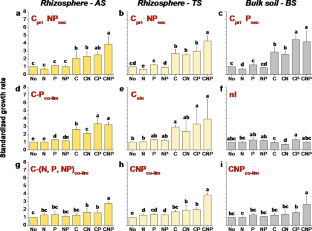
Explore related subjects
- Environmental Chemistry
Data availability
The datasets analyzed in the current study are available from the corresponding author on reasonable request.
Browning TJ, Achterberg EP, Rapp I, Engel A, Bertrand EM, Tagliabue A, Moore CM (2017) Nutrient co-limitation at the boundary of an oceanic gyre. Nature 551:242–246
Article CAS PubMed Google Scholar
Chen J, Jia B, Gang S, Li Y, Li F-C, Mou XM, Kuzyakov Y, Li XG (2022) Decoupling of soil organic carbon and nutrient mineralization across plant communities as affected by microbial stoichiometry. Biol Fertil Soils 58:693–706
Article CAS Google Scholar
Dai T, Wen D, Bates CT, Wu L, Guo X, Liu S, Su Y, Lei J, Zhou J, Yang Y (2022) Nutrient supply controls the linkage between species abundance and ecological interactions in marine bacterial communities. Nat Commun 13:175
Article CAS PubMed PubMed Central Google Scholar
Demoling F, Figueroa D, Bååth E (2007) Comparison of factors limiting bacterial growth in different soils. Soil Biol Biochem 39:2485–2495
Dijkstra FA, Zhu B, Cheng W (2021) Root effects on soil organic carbon: a double-edged sword. New Phytol 230:60–65
Drake JE, Gallet-Budynek A, Hofmockel KS, Bernhardt ES, Billings SA, Jackson RB, Johnsen KS, Lichter J, McCarthy HR, McCormack ML, Moore DJP, Oren R, Palmroth S, Phillips RP, Pippen JS, Pritchard SG, Treseder KK, Schlesinger WH, DeLucia EH, Finzi AC (2011) Increases in the flux of carbon belowground stimulate nitrogen uptake and sustain the long-term enhancement of forest productivity under elevated CO 2 . Ecol Lett 14:349–357
Article PubMed Google Scholar
Du E, Terrer C, Pellegrini AFA, Ahlström A, van Lissa CJ, Zhao X, Xia N, Wu X, Jackson RB (2020) Global patterns of terrestrial nitrogen and phosphorus limitation. Nat Geosci 13:221–226
Finzi AC, Abramoff RZ, Spiller KS, Brzostek ER, Darby BA, Kramer MA, Phillips RP (2015) Rhizosphere processes are quantitatively important components of terrestrial carbon and nutrient cycles. Glob Chang Biol 21:2082–2094
Kuzyakov Y, Blagodatskaya E (2015) Microbial hotspots and hot moments in soil: Concept & review. Soil Biol Biochem 83:184–199
Lee H, Schuur EAG, Inglett KS, Lavoie M, Chanton JP (2012) The rate of permafrost carbon release under aerobic and anaerobic conditions and its potential effects on climate. Glob Chang Biol 18:515–527
Article Google Scholar
Lehmann J, Kleber M (2015) The contentious nature of soil organic matter. Nature 528:60–68
McCormack ML, Dickie IA, Eissenstat DM, Fahey TJ, Fernandez CW, Guo D, Helmisaari H-S, Hobbie EA, Iversen CM, Jackson RB, Leppälammi-Kujansuu J, Norby RJ, Phillips RP, Pregitzer KS, Pritchard SG, Rewald B, Zadworny M (2015) Redefining fine roots improves understanding of below-ground contributions to terrestrial biosphere processes. New Phytol 207:505–518
Nazari M, Bickel S, Kuzyakov Y, Bilyera N, Zarebanadkouki M, Wassermann B, Dippold MA (2024) Root mucilage nitrogen for rhizosphere microorganisms under drought. Biol Fertil Soils 60:639–647
Pan W, Zhou J, Tang S, Wu L, Ma Q, Marsden KA, Chadwick DR, Jones DL (2023) Utilisation and transformation of organic and inorganic nitrogen by soil microorganisms and its regulation by excessive carbon and nitrogen availability. Biol Fertil Soils 59:379–389
Phillips RP, Meier IC, Bernhardt ES, Grandy AS, Wickings K, Finzi AC (2012) Roots and fungi accelerate carbon and nitrogen cycling in forests exposed to elevated CO 2 . Ecol Lett 15:1042–1049
Qiu Q, Li M, Mgelwa AS, Hu Y-L (2023) Divergent mineralization of exogenous organic substrates and their priming effects depending on soil types. Biol Fertil Soils 59:87–101
Sinsabaugh RL, Hill BH, Shah JJF (2009) Ecoenzymatic stoichiometry of microbial organic nutrient acquisition in soil and sediment. Nature 462:795–798
Soong JL, Fuchslueger L, Marañon-Jimenez S, Torn MS, Janssens IA, Penuelas J, Richter A (2020) Microbial carbon limitation: the need for integrating microorganisms into our understanding of ecosystem carbon cycling. Glob Chang Biol 26:1953–1961
Spohn M, Kuzyakov Y (2013) Phosphorus mineralization can be driven by microbial need for carbon. Soil Biol Biochem 61:69–75
Spohn M, Klaus K, Wanek W, Richter A (2016) Microbial carbon use efficiency and biomass turnover times depending on soil depth – implications for carbon cycling. Soil Biol Biochem 96:74–81
Treseder KK (2008) Nitrogen additions and microbial biomass: a meta-analysis of ecosystem studies. Ecol Lett 11:1111–1120
Wang C, Kuzyakov Y (2023) Energy use efficiency of soil microorganisms: driven by carbon recycling and reduction. Glob Chang Biol 29:6170–6187
Wang J, Wu Y, Zhou J, Bing H, Sun H, He Q, Li J, Wilcke W (2020) Soil microbes become a major pool of biological phosphorus during the early stage of soil development with little evidence of competition for phosphorus with plants. Plant Soil 446:259–274
Wang Q, Zhang Z, Guo W, Zhu X, Xiao J, Liu Q, Yin H (2021) Absorptive and transport roots differ in terms of their impacts on rhizosphere soil carbon storage and stability in alpine forests. Soil Biol Biochem 161:108379
Wang X, Chen R, Petropoulos E, Yu B, Lin X, Feng Y (2023) Root-derived C distribution drives N transport and transformation after 13 C and 15 N labelling on paddy and upland soils. Biol Fertil Soils 59:513–525
Zhang Z, Yuan Y, Zhao W, He H, Li D, He W, Liu Q, Yin H (2017) Seasonal variations in the soil amino acid pool and flux following the conversion of a natural forest to a pine plantation on the eastern tibetan Plateau, China. Soil Biol Biochem 105:1–11
Zhu X, Lambers H, Guo W, Chen D, Liu Z, Zhang Z, Yin H (2023) Extraradical hyphae exhibit more plastic nutrient-acquisition strategies than roots under nitrogen enrichment in ectomycorrhiza-dominated forests. Glob Chang Biol 29:4605–4619
Download references
Acknowledgements
This study was supported jointly by the National Natural Science Foundation of China (U23A2051, 32201531, 32301446 and 32171757), the Chinese Academy of Sciences (CAS) Interdisciplinary Innovation Team (xbzg-zysys-202112), the Science and technology program of Tibet Autonomous Region (XZ202301YD0028C and XZ202301ZR0047G), and Sichuan Science and Technology Program (2023NSFSC0012 and 2023NSFSC1192). The authors highly appreciate the constructive comments from Editor-in-Chief Paolo Nannipieri and two anonymous reviewers, which have greatly improved the quality of this paper.
Author information
Authors and affiliations.
CAS Key Laboratory of Mountain Ecological Restoration and Bioresource Utilization & Ecological Restoration and Biodiversity Conservation Key Laboratory of Sichuan Province & China-Croatia “Belt and Road” Joint Laboratory on Biodiversity and Ecosystem Services, Chengdu Institute of Biology, Chinese Academy of Sciences, Chengdu, 610213, China
Jipeng Wang, Min Li, Qitong Wang, Dungang Wang, Peipei Zhang, Na Li & Huajun Yin
School of Ecology and Environment, Northwestern Polytechnical University, Xi’an, 710072, China
Ziliang Zhang
College of Ecology and Environment, Chengdu University of Technology, Chengdu, 610059, China
Yiqiu Zhong
You can also search for this author in PubMed Google Scholar
Corresponding author
Correspondence to Huajun Yin .
Ethics declarations
Conflict of interest.
The authors declare no competing interests.
Additional information
Publisher’s note.
Springer Nature remains neutral with regard to jurisdictional claims in published maps and institutional affiliations.
Electronic supplementary material
Below is the link to the electronic supplementary material.
Supplementary Material 1
Rights and permissions.
Reprints and permissions
About this article
Wang, J., Li, M., Wang, Q. et al. Full-factorial resource amendment experiments reveal carbon limitation of rhizosphere microbes in alpine coniferous forests. Biol Fertil Soils (2024). https://doi.org/10.1007/s00374-024-01860-7
Download citation
Received : 12 May 2024
Revised : 20 August 2024
Accepted : 22 August 2024
Published : 05 September 2024
DOI : https://doi.org/10.1007/s00374-024-01860-7
Share this article
Anyone you share the following link with will be able to read this content:
Sorry, a shareable link is not currently available for this article.
Provided by the Springer Nature SharedIt content-sharing initiative
- Resource limitation
- Absorptive and transport roots
- Microbial growth
- Microbial respiration
- Plant-microbial interaction
- Find a journal
- Publish with us
- Track your research
IMAGES
VIDEO
COMMENTS
Factorial experiment
14.2: Design of experiments via factorial designs
In many factorial designs, one of the independent variables is a non-manipulated independent variable. The researcher measures it but does not manipulate it. The study by Schnall and colleagues is a good example. One independent variable was disgust, which the researchers manipulated by testing participants in a clean room or a messy room.
A full factorial design (also known as complete factorial design) is the most complete of the design options, meaning that each factor and level are combined to test every possible combination condition. Let us expand upon the theoretical ERAS factorial experiment as an illustrative example. We designed our own ERAS protocol for Whipple procedures, and our objective is to test which components ...
3.1: Factorial Designs
Coding Systems for the Factor Levels in the Factorial Design of Experiment. As the factorial design is primarily used for screening variables, only two levels are enough. Often, coding the levels as (1) low/high, (2) -/+ or (3) -1/+1 is more convenient and meaningful than the actual level of the factors, especially for the designs and analyses ...
5.2.6. Main Effects and Interactions. In factorial designs, there are two kinds of results that are of interest: main effects and interactions. A main effect is the statistical relationship between one independent variable and a dependent variable-averaging across the levels of the other independent variable (s).
A factorial design study uses more than one independent variable or factor. This design allows researchers to look at how multiple factors affect a dependent variable, both independently and together. Factorial design studies are titled by the number of levels of the factors. For example, a study with two factors that each have two levels is ...
Experiments of factorial design offer a highly efficient method to evaluate multiple component interventions. The main effect of multiple components can be measured with the same number of participants as a classic two-arm randomized controlled trial (RCT) while maintaining adequate statistical power. In addition, interactions between components can be estimated.
How a Factorial Design Works. Let's take a closer look at how a factorial design might work in a psychology experiment: The independent variable is the variable of interest that the experimenter will manipulate.; The dependent variable is the variable that the researcher then measures.; By doing this, psychologists can see if changing the independent variable results in some type of change ...
Topic 9. Factorial Experiments [ST&D Chapter 15]
Figure 9.1 Factorial Design Table Representing a 2 × 2 Factorial Design. In principle, factorial designs can include any number of independent variables with any number of levels. For example, an experiment could include the type of psychotherapy (cognitive vs. behavioral), the length of the psychotherapy (2 weeks vs. 2 months), and the sex of ...
A Complete Guide: The 2x2 Factorial Design
Factorial Experiment
For analysis of. 2n. factorial experiment, the analysis of variance involves the partitioning of treatment sum of squares so as to obtain sum of squares due to main and interaction effects of factors. These sum of squares are mutually orthogonal, so Treatment SS = Total of SS due to main and interaction effects.
ORIAL DESIGNS4.1 Two Factor Factorial DesignsA two-factor factorial design is an experimental design in which data is collected for all possible combination. sible factor combinations then the de. ign is abalanced two-factor factorial design.A balanced a b factorial design is a factorial design for which there are a levels of factor A, b levels ...
Answer: We learn the population means by estimating the common variance 2 in two di erent ways. These two estimators are formed by. measuring variability of the observations within each sample. measuring variability of the sample means across the samples. Idea: These two estimates tend to be similar when H0 is true.
Factor 1: three pulp preparation methods Factor 2: four cooking temperatures. Objective: study the effect on the tensile strength of the paper. Three replicates of a 4 ‚ 3 experiment A batch of pulp is produced by one of the three methods; then it is divided into 4 samples. Each sample is cooked at one temperature.
Formally, main effects are the mean differences for a single Independent variable. There is always one main effect for each IV. A 2x2 design has 2 IVs, so there are two main effects. In our example, there is one main effect for distraction, and one main effect for reward. We will often ask if the main effect of some IV is significant.
A mean square is an estimate of population variance. It is computed by dividing a sum of squares (SS) by its corresponding degrees of freedom (df), as shown below: MS = SS / df. To conduct analysis of variance with a two-factor, full factorial experiment, we are interested in four mean squares: Factor A mean square.
In many factorial designs, one of the independent variables is a non-manipulated independent variable. The researcher measures it but does not manipulate it. The study by Schnall and colleagues is a good example. One independent variable was disgust, which the researchers manipulated by testing participants in a clean room or a messy room.
Experimental Design: Types, Examples & Methods
Together, these suggest the QALY may be a flawed measure of the value of EOL care. To test these arguments, we administered a stated preference survey in a UK-representative public sample. ... Factorial Survey Experiments. 2015. View more. Open in viewer. Go to. Go to. Show all references. Request permissions Show all. Collapse. Expand Table.
The high permeability of gravel sand increases the risk of water spewing from the screw conveyor during earth pressure balance (EPB) shield tunnelling. The effectiveness of soil conditioning is a key factor affecting EPB shield tunnelling and construction safety. In this paper, using polymer, a foaming agent, and bentonite slurry as conditioning additives, the permeability coefficient tests of ...
On Sunday, Measure 110, Oregon's 3 1/2-year experiment will come to an end, and possession of small amounts of drugs will once again be considered a misdemeanor crime. Fed-up residents say it ...
The measure required officers to hand out $100 citations instead of jail time, and that citation could be waived if the person called a state-funded hotline and enrolled in an assessment for ...
Oregon has ended its experiment with drug decriminalization. Starting Sept. 1, possession of small amounts of illicit substances are once again considered a misdemeanor crime.
We conducted a full-factorial resource addition experiment to identify the limiting resources of microbial growth and respiration according to Demoling et al ... A repeated measures ANOVA, with soil compartment as the within-subjects factor and site as the between-subjects factor, was used to detect the differences between soil compartments and ...